Take-home Exercise 3 (Revised): Exploratory Spatial Data Analysis for Potential Push & Pull Factors of Locations in Singapore using Public Bus Data

Author

Victoria Grace ANN

Published

March 11, 2024

Modified

March 31, 2024

1.0 Overview

In this exercise, my focus would be on prototyping exploratory spatial data analysis, particularly density of spatial assets within hexagonal traffic analysis zones. In conventional geography, a traffic analysis zone is the unit most commonly used in transportation planning models and the size of it varies. Hexagonal traffic analysis zones has gained traction as the hexagons of the study area have a uniform size which are easily comparable with each other when determining transport attractiveness. It is also recommended that hexagon radius should be 125m for areas in high urbanisation and 250m in areas with less urbanisation (Chmielewski et al., 2020).

The data preparation for this purpose also supports the preparation for calibrating spatial interaction models. For the prototyping, only exploratory spatial data analysis will be done.

2.0 Package Installation

I will load up the below R packages for the following purposes:

tmap: to visualise spatial data by creating thematic maps that could be interactive or static.
sf: to manipulate spatial data.
sp: to manipulate spatial data (older than sp).
reshape2: to reshape and transform data frames; converting data between “wide” and “long” formats using functions like melt().
ggplot2: to visualise data with plot types including bar plots.
tidyverse: to clean and transform data and contains sub-packagess including tidyr, dplyr and readr.
stplanr: to provide functions suitable for working with spatial transport data like networks, orgins-destinations matrices and travel time matrices; builds on the capabilities of sf and sp packages.
knitr: to combine code into a single documents that can be easily converted to various output formats like html, pdf, or Word.
kableExtra: to further style any Kables.
spdep: to create spatial wieght matrix objects from contiguities
spflow: to estimate spatial econometric interaction models

pacman::p_load(tmap, sf, sp, reshape2, ggplot2, ggpubr, tidyverse, stplanr, knitr, kableExtra, spdep)

devtools::install_github("LukeCe/spflow")
library(spflow)

3.0 Data sources

URA’s Masterplan Subzone 2019 Layer in shapefile format
Bus Stop Locations extracted from LTA
A tabulated bus passenger flow for Nov 2023, Dec 2023 and Jan 2024 from LTA dynamic data mall
Population Data for 2023 from SingStat
Schools from MOE
Financial Services
Hospitals, polyclinics and CHAS clinics derived from Google Maps

4.0 Data preparation

4.1 Data preparation for bus-induced hexagons

Read the subzone layer

mpsz <- st_read("data/geospatial/master-plan-2019-subzone-boundary-no-sea-kml.kml")

Convert mpsz to 2D geometry.

mpsz <- st_zm(mpsz, drop = TRUE) # Convert 3D geometries to 2D

Extract the SUBZONE_N and PLN_AREA_N from the Dscrptn field

For SUBZONE_N,

mpsz <- mpsz %>%
  rowwise() %>%
  mutate(SUBZONE_N = str_extract(Description, "<th>SUBZONE_N</th> <td>(.*?)</td>")) %>%
  ungroup()

mpsz$SUBZONE_N <- str_remove_all(mpsz$SUBZONE_N, "<.*?>|SUBZONE_N")

For PLN_AREA_N,

mpsz <- mpsz %>%
  rowwise() %>%
  mutate(PLN_AREA_N = str_extract(Description, "<th>PLN_AREA_N</th> <td>(.*?)</td>")) %>%
  ungroup()

mpsz$PLN_AREA_N <- str_remove_all(mpsz$PLN_AREA_N, "<.*?>|PLN_AREA_N")

Remove the Description column.

mpsz$Description <- NULL

Remove unwanted outer islands.

mpsz3414 <- mpsz %>% st_transform(crs = 3414)

outer_islands <- c("SEMAKAU", "SUDONG", "NORTH-EASTERN ISLANDS", "SOUTHERN GROUP")
mpsz3414 <- mpsz3414 %>%
  filter(!str_trim(SUBZONE_N) %in% str_trim(outer_islands))

Create the shapefile.

st_write(mpsz3414, "data/geospatial/mpsz3414.shp", append=FALSE)

Read the updated shapefile.

mpsz3414 <- st_read("data/geospatial/mpsz3414.shp")

Reading layer `mpsz3414' from data source 
  `C:\guacodemoleh\IS415-GAA\Take-home_Ex\Take-home_Ex03\data\geospatial\mpsz3414.shp' 
  using driver `ESRI Shapefile'
Simple feature collection with 328 features and 3 fields
Geometry type: MULTIPOLYGON
Dimension:     XY
Bounding box:  xmin: 2667.538 ymin: 21448.47 xmax: 55941.94 ymax: 50256.33
Projected CRS: SVY21 / Singapore TM

Read the aspatial bus stop layer and set its CRS to 3414.

BusStop <- read.csv("data/aspatial/bus_coords_subzone_v2.csv") %>% st_as_sf(coords=c("Longitude", "Latitude"), crs=4326) %>%
  st_transform(crs=3414)

summary(BusStop)

  BusStopCode      RoadName         Description          Subzone         
 Min.   : 1012   Length:5107        Length:5107        Length:5107       
 1st Qu.:25345   Class :character   Class :character   Class :character  
 Median :49031   Mode  :character   Mode  :character   Mode  :character  
 Mean   :48663                                                           
 3rd Qu.:67065                                                           
 Max.   :99189                                                           
          geometry   
 POINT        :5107  
 epsg:3414    :   0  
 +proj=tmer...:   0

Ensure that all bus stops are within Singapore’s boundary.

BusStop <- BusStop %>% st_intersection(mpsz3414) %>% select(BusStopCode, )

tm_shape(mpsz3414) +
  tm_polygons() +
  tm_shape(BusStop) +
  tm_dots()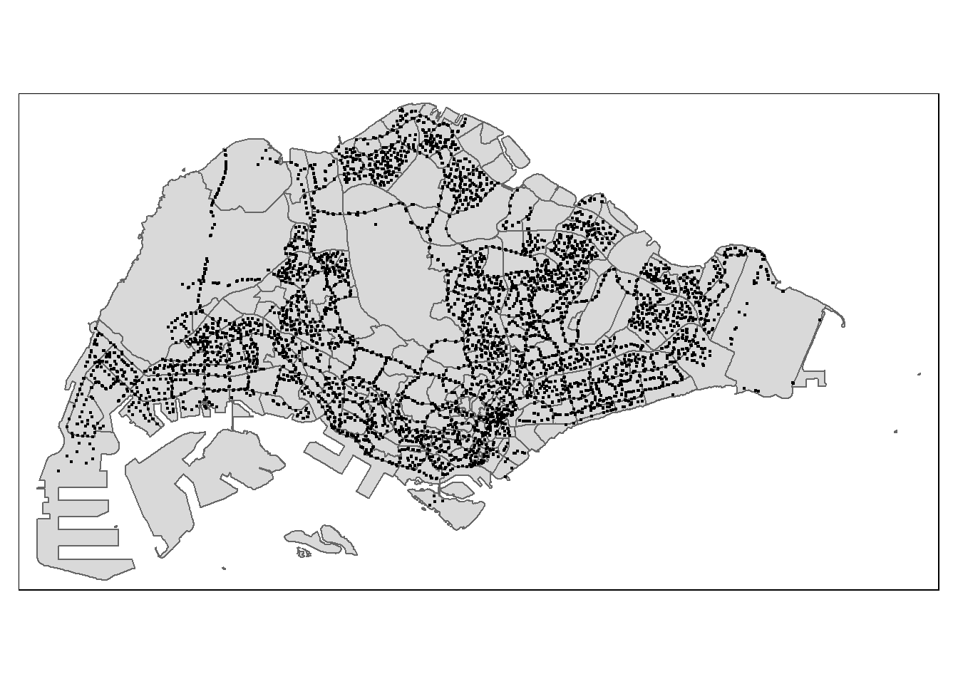

Generate the hexagon grids using st_make_grid() with a cellsize of 750m.

hex_grids <- BusStop %>% st_make_grid(cellsize =750,
                                       what = "polygons",
                                       square = FALSE) %>%
  st_sf() %>%
  filter(lengths(st_intersects(geometry, BusStop)) > 0)

Code interpretation

st_make_grid: creates grids covering areas also without bus stops
cellsize: hexagon size determined by twice the length of the apothem
st_sf: set the hexagons as a sf object
filter: filtering for hexagons that contain bus stops

Have a look and check if the hexagons cover all the bus stop locations.

tm_shape(mpsz3414) +
  tm_polygons(title = "Singapore Boundary") +
  tm_shape(hex_grids) +
  tm_polygons(col = "white", title = "Hexagons", alpha = 1) +
  tm_layout(main.title = "Hexagons corresponding to Singapore bus stops",
            main.title.position = "center",
            main.title.size = 1.0,
            legend.height = 0.35, 
            legend.width = 0.35,
            frame = TRUE) +
  tm_compass(type="8star", size = 2, bg.color = "white", bg.alpha = 0.5) +
  tm_scale_bar(bg.color = "white", bg.alpha = 0.5) +
  tm_shape(BusStop) +
  tm_dots(col = "red", size = 0.001, title = "Bus Stops") +
  tm_grid(alpha = 0.2)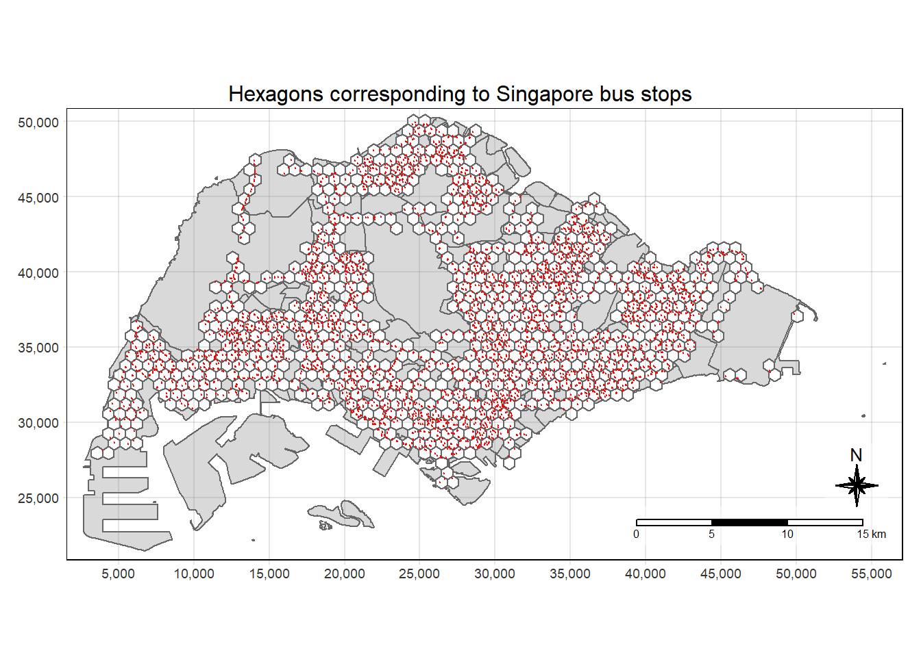

Assign ID to each hexagon

Each hexagon will have an assigned ID that will be their unique identifier. This new information can be stored under the HEX_ID column which will be helpful for joining data frames.

hex_grids$HEX_ID <- sprintf("H%04d", seq_len(nrow(hex_grids))) %>%
  as.factor()

Save the layer

write_rds(hex_grids, "data/rds/hex_grids.rds")

hex_grids <- read_rds("data/rds/hex_grids.rds")

kable(head(hex_grids))

geometry	HEX_ID
POLYGON ((3578.167 27517.51…	H0001
POLYGON ((4328.167 27517.51…	H0002
POLYGON ((4328.167 28816.55…	H0003
POLYGON ((4328.167 30115.59…	H0004
POLYGON ((4703.167 28167.03…	H0005
POLYGON ((4703.167 29466.07…	H0006

4.2 Spatial Interaction Analysis

Combining OD data

od_bus_nov <- read_csv("data/OD Bus/merged_bus_nov_v2.csv")
od_bus_dec <- read_csv("data/OD Bus/merged_bus_dec_v2.csv")
od_bus_jan <- read_csv("data/OD Bus/merged_bus_jan_v2.csv")

OD <- rbind(od_bus_nov, od_bus_dec)
OD <- rbind(OD, od_bus_jan)

nrow(od_bus_nov) + nrow(od_bus_dec) + nrow(od_bus_jan) == nrow(OD) # evaluates to TRUE

str(OD)

ORIGIN_PT_CODE and DESTINATION_PT_CODE are listed as character variables. These variables should be transformed to factors so that R treats them as grouping variables.

cols_to_convert <- c("ORIGIN_PT_CODE", "DESTINATION_PT_CODE")

OD[cols_to_convert] <- lapply(OD[cols_to_convert], as.factor)

glimpse(OD)

ORIGIN_PT_CODEandDESTINATION_PT_CODE` are now factors.

write_rds(OD, "data/rds/odbus_combined.rds")

odbus_combined <- read_rds("data/rds/odbus_combined.rds")

Creating Commute Flow Data

od <- odbus_combined %>%
  group_by(ORIGIN_PT_CODE, ORIGIN_SUBZONE, DESTINATION_PT_CODE, DESTINATION_SUBZONE, DAY_TYPE ,TIME_PER_HOUR) %>%
  summarise(TRIPS = sum(TOTAL_TRIPS)) %>%
  ungroup()

write_rds(od, "data/rds/od.rds")

od <- read_rds("data/rds/od.rds")

Generating O-D trip data by hexagon level

We can create a lookup table for the bus stops associated to each hexagon.

Generating lookup table for bus stop to associated hexagon

To connect the trip data to their corresponding hexagons, a lookup table needs to be made so that there is a relationship beetween the aspatial od and hex_grids.

bs_hex <- st_intersection(BusStop, hex_grids) %>%
  st_drop_geometry() %>%
  select(c(BusStopCode, HEX_ID))

kable(head(bs_hex))

	BusStopCode	HEX_ID
1241	25059	H0001
1241.1	25059	H0002
1341	25751	H0003
1395	26379	H0004
1342	25761	H0005
1337	25711	H0006

Multiple HEX_ID per bus stop

Some bus stops may fall in the boundary of neighbouring hexagons. To resolve this, such bus stops shall be assigned to the first identified corresponding HEX_ID.

bs_hex <- bs_hex %>%
  group_by(BusStopCode) %>%
  summarise(across(everything(), first)) %>%
  ungroup()

nrow(bs_hex) == nrow(BusStop)

[1] TRUE

Joining od and bs_hex

Associate the origin bus stops and destination bus stops to their corresponding hexagons.

bs_hex$BusStopCode <- as.factor(bs_hex$BusStopCode)

od_trips_w_hex <- od %>%
  inner_join(bs_hex,
             by = c("ORIGIN_PT_CODE" = "BusStopCode")) %>%
  rename(ORIG_HEX_ID = HEX_ID) %>%
  inner_join(bs_hex,
             by = c("DESTINATION_PT_CODE" = "BusStopCode")) %>%
  rename(DEST_HEX_ID = HEX_ID)

kable(head(od_trips_w_hex))

ORIGIN_PT_CODE	ORIGIN_SUBZONE	DESTINATION_PT_CODE	DESTINATION_SUBZONE	DAY_TYPE	TIME_PER_HOUR	TRIPS	ORIG_HEX_ID	DEST_HEX_ID
10009	BUKIT MERAH	10017	BUKIT MERAH	WEEKDAY	5	9	H0381	H0455
10009	BUKIT MERAH	10017	BUKIT MERAH	WEEKDAY	7	5	H0381	H0455
10009	BUKIT MERAH	10017	BUKIT MERAH	WEEKDAY	8	2	H0381	H0455
10009	BUKIT MERAH	10017	BUKIT MERAH	WEEKDAY	9	29	H0381	H0455
10009	BUKIT MERAH	10017	BUKIT MERAH	WEEKDAY	10	11	H0381	H0455
10009	BUKIT MERAH	10017	BUKIT MERAH	WEEKDAY	11	14	H0381	H0455

::: {,callout-warning collapse=“true”} ### Save Data Memory Space

od is not needed anymore since the necessary data has been extracted, so we can offload it.

rm(od)

Aggregating data by hexagon

Perform aggregations by ORIGIN_HEX_ID and DEST_HEX_ID to have an aggregated sum of trips by hexagon instead of bus stops.

od_hex <- od_trips_w_hex %>%
  group_by(ORIG_HEX_ID, ORIGIN_SUBZONE ,DEST_HEX_ID, DESTINATION_SUBZONE, DAY_TYPE, TIME_PER_HOUR) %>%
  summarise(TRIPS = sum(TRIPS))

kable(head(od_hex))

ORIG_HEX_ID	ORIGIN_SUBZONE	DEST_HEX_ID	DESTINATION_SUBZONE	DAY_TYPE	TIME_PER_HOUR	TRIPS
H0001	TUAS	H0005	TUAS	WEEKDAY	18	2
H0001	TUAS	H0006	TUAS	WEEKDAY	7	2
H0001	TUAS	H0006	TUAS	WEEKDAY	8	9
H0001	TUAS	H0006	TUAS	WEEKDAY	12	1
H0001	TUAS	H0006	TUAS	WEEKDAY	16	1
H0001	TUAS	H0006	TUAS	WEEKDAY	17	1

Save the layer

write_rds(bs_hex, "data/rds/bs_hex.rds")
write_rds(od_hex, "data/rds/od_hex.rds")

Generating flow lines

od_hex <- od_hex[, c(1, 3, 2, 4:ncol(od_hex))]

flowlines <- od_hex %>% od2line(
  hex_grids,
  zone_code = "HEX_ID")

write_rds(flowlines, "data/rds/flowlines.rds")

Learning Point

The flow data in the od2line function must have the origin and destination indexes in its first two columns.

flowlines <- read_rds("data/rds/flowlines.rds")

Inspect flowlines

Large data size

The flowlines data is very large.

For all visualisations, the number of trips per flowline shown will be 3000 and above.

tm_shape(mpsz3414) +
  tm_polygons(title = "Singapore Boundary", alpha = 0.5) +
  
  tm_shape(hex_grids) +
  tm_polygons(col = "white", title = "Hexagons", alpha = 1) +
  
  tm_shape(flowlines[flowlines$TRIPS >= 3000,]) +
  tm_lines(lwd = "TRIPS",
           style = "quantile",
           col = "red",
           scale = c(0.1, 1, 3, 5, 7),
           title.lwd = "# of bus trips",
           alpha = 0.8) +
  
  tm_layout(main.title = "Overall Bus Passenger Flow for Weekdays)",
            main.title.position = "center",
            main.title.size = 1.0,
            legend.height = 0.35, 
            legend.width = 0.35,
            frame = TRUE) +
  
  tm_compass(type="8star", size = 2, bg.color = "white", bg.alpha = 0.5) +
  tm_scale_bar(bg.color = "white", bg.alpha = 0.5) +
  tm_grid(alpha = 0.2)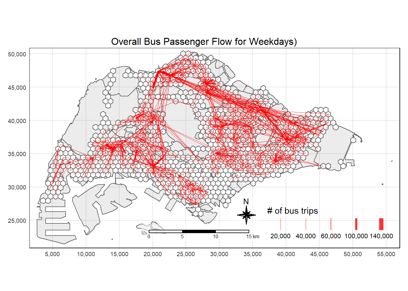

Save Data Memory

rm(flowlines)
rm(od_hex)

4.2.1 Prototype for Spatial Interaction Analysis

5.0 Spatial Interaction Modelling

5.1.1 Attractiveness variables

Initiate the attractiveness from hex_grids.

attractiveness <- hex_grids %>% st_set_crs(3414)

For all the variables, we only need to count the number of each location types per hexagon, which can be done using lengths() and st_intersects().

POIs

attractiveness$BUS_STOP_COUNT <- lengths(
  st_intersects(attractiveness, BusStop))

entertn <- st_read("data/geospatial/entertn.shp") %>% st_set_crs(3414)

Reading layer `entertn' from data source 
  `C:\guacodemoleh\IS415-GAA\Take-home_Ex\Take-home_Ex03\data\geospatial\entertn.shp' 
  using driver `ESRI Shapefile'
Simple feature collection with 114 features and 3 fields
Geometry type: POINT
Dimension:     XY
Bounding box:  xmin: 10809.34 ymin: 26528.63 xmax: 41600.62 ymax: 46375.77
Projected CRS: SVY21 / Singapore TM

attractiveness$ENTERTN_COUNT <- lengths(st_intersects(attractiveness, entertn))

food_bev <- st_read("data/geospatial/F&B.shp") %>% st_set_crs(3414)

Reading layer `F&B' from data source 
  `C:\guacodemoleh\IS415-GAA\Take-home_Ex\Take-home_Ex03\data\geospatial\F&B.shp' 
  using driver `ESRI Shapefile'
Simple feature collection with 1919 features and 3 fields
Geometry type: POINT
Dimension:     XY
Bounding box:  xmin: 6010.495 ymin: 25343.27 xmax: 45462.43 ymax: 48796.21
Projected CRS: SVY21 / Singapore TM

attractiveness$FOOD_BEV_COUNT <- lengths(st_intersects(attractiveness, food_bev))

leis_rec <- st_read("data/geospatial/Liesure&Recreation.shp") %>% st_set_crs(3414)

Reading layer `Liesure&Recreation' from data source 
  `C:\guacodemoleh\IS415-GAA\Take-home_Ex\Take-home_Ex03\data\geospatial\Liesure&Recreation.shp' 
  using driver `ESRI Shapefile'
Simple feature collection with 1217 features and 30 fields
Geometry type: POINT
Dimension:     XY
Bounding box:  xmin: 6010.495 ymin: 25134.28 xmax: 48439.77 ymax: 50078.88
Projected CRS: SVY21 / Singapore TM

attractiveness$LEISURE_COUNT <- lengths(st_intersects(attractiveness, leis_rec))

retail <- st_read("data/geospatial/Retails.shp") %>% st_set_crs(3414)

Reading layer `Retails' from data source 
  `C:\guacodemoleh\IS415-GAA\Take-home_Ex\Take-home_Ex03\data\geospatial\Retails.shp' 
  using driver `ESRI Shapefile'
Simple feature collection with 37635 features and 3 fields
Geometry type: POINT
Dimension:     XY
Bounding box:  xmin: 4737.982 ymin: 25171.88 xmax: 48265.04 ymax: 50135.28
Projected CRS: SVY21 / Singapore TM

attractiveness$RETAIL_COUNT <- lengths(st_intersects(attractiveness, retail))

biz <- st_read("data/geospatial/Business.shp") %>% st_set_crs(3414)

Reading layer `Business' from data source 
  `C:\guacodemoleh\IS415-GAA\Take-home_Ex\Take-home_Ex03\data\geospatial\Business.shp' 
  using driver `ESRI Shapefile'
Simple feature collection with 6550 features and 3 fields
Geometry type: POINT
Dimension:     XY
Bounding box:  xmin: 3669.148 ymin: 25408.41 xmax: 47034.83 ymax: 50148.54
Projected CRS: SVY21 / Singapore TM

attractiveness$BIZ_COUNT <- lengths(st_intersects(attractiveness, biz))

fin <- st_read("data/geospatial/FinServ.shp") %>% st_set_crs(3414)

Reading layer `FinServ' from data source 
  `C:\guacodemoleh\IS415-GAA\Take-home_Ex\Take-home_Ex03\data\geospatial\FinServ.shp' 
  using driver `ESRI Shapefile'
Simple feature collection with 3320 features and 3 fields
Geometry type: POINT
Dimension:     XY
Bounding box:  xmin: 4881.527 ymin: 25171.88 xmax: 46526.16 ymax: 49338.02
Projected CRS: SVY21 / Singapore TM

attractiveness$FIN_COUNT <- lengths(st_intersects(attractiveness, fin))

Data preparation

hdb <- read_csv("data/aspatial/hdb.csv")

For the purpose of computing a proxy for population density, the residential units will be extracted using filter() from the dplyr package.

hdb_residential <- hdb %>%
  filter(residential == "Y")

head(hdb_residential, 10)

# A tibble: 10 × 37
    ...1 blk_no street       max_floor_lvl year_completed residential commercial
   <dbl> <chr>  <chr>                <dbl>          <dbl> <chr>       <chr>     
 1     0 1      BEACH RD                16           1970 Y           Y         
 2     1 1      BEDOK STH A…            14           1975 Y           N         
 3     3 1      CHAI CHEE RD            15           1982 Y           N         
 4     4 1      CHANGI VILL…             4           1975 Y           Y         
 5     5 1      DELTA AVE               25           1982 Y           N         
 6     6 1      DOVER RD                12           1975 Y           N         
 7     7 1      EUNOS CRES              14           1977 Y           N         
 8     8 1      EVERTON PK              12           1980 Y           Y         
 9    10 1      GHIM MOH RD             15           1975 Y           N         
10    11 1      HAIG RD                 15           1976 Y           N         
# ℹ 30 more variables: market_hawker <chr>, miscellaneous <chr>,
#   multistorey_carpark <chr>, precinct_pavilion <chr>,
#   bldg_contract_town <chr>, total_dwelling_units <dbl>, `1room_sold` <dbl>,
#   `2room_sold` <dbl>, `3room_sold` <dbl>, `4room_sold` <dbl>,
#   `5room_sold` <dbl>, exec_sold <dbl>, multigen_sold <dbl>,
#   studio_apartment_sold <dbl>, `1room_rental` <dbl>, `2room_rental` <dbl>,
#   `3room_rental` <dbl>, other_room_rental <dbl>, lat <dbl>, lng <dbl>, …

There are also some outliers like hotels that are classified as a residential unit. We can remove rows containing ‘hotel’ using grepl().

hotels <- hdb_residential %>%
  filter(grepl("HOTEL", building, ignore.case = TRUE))

kable(hotels)

…1	blk_no	street	max_floor_lvl	year_completed	residential	commercial	market_hawker	miscellaneous	multistorey_carpark	precinct_pavilion	bldg_contract_town	total_dwelling_units	1room_sold	2room_sold	3room_sold	4room_sold	5room_sold	exec_sold	multigen_sold	studio_apartment_sold	1room_rental	2room_rental	3room_rental	other_room_rental	lat	lng	building	addr	postal	SUBZONE_NO	SUBZONE_N	SUBZONE_C	PLN_AREA_N	PLN_AREA_C	REGION_N	REGION_C
0	1	BEACH RD	16	1970	Y	Y	N	N	N	N	KWN	142	0	1	138	1	2	0	0	0	0	0	0	0	1.295097	103.8541	RAFFLES HOTEL	1 BEACH ROAD RAFFLES HOTEL SINGAPORE 189673	189673	2	CITY HALL	DTSZ02	DOWNTOWN CORE	DT	CENTRAL REGION	CR
4580	3	BEACH RD	16	1970	Y	Y	N	N	N	N	KWN	138	0	1	134	0	3	0	0	0	0	0	0	0	1.294801	103.8545	RAFFLES HOTEL SINGAPORE	3 BEACH ROAD RAFFLES HOTEL SINGAPORE SINGAPORE 189674	189674	2	CITY HALL	DTSZ02	DOWNTOWN CORE	DT	CENTRAL REGION	CR

The HDB Blk 1 Beach Road shares a similar address as Raffles Hotel’s 1 Beach Road, but they have different postal codes.

To verify other similar addresses, filter for addresses containing “BEACH RD”.

beach_rd <- hdb_residential %>%
  filter(grepl("BEACH RD", street, ignore.case = TRUE))

kable(beach_rd)

…1	blk_no	street	max_floor_lvl	year_completed	residential	commercial	market_hawker	miscellaneous	multistorey_carpark	precinct_pavilion	bldg_contract_town	total_dwelling_units	2room_sold	3room_sold	4room_sold	5room_sold	1room_rental	2room_rental	lat	lng	building	addr	postal	SUBZONE_NO	SUBZONE_N	SUBZONE_C	PLN_AREA_N	PLN_AREA_C	REGION_N	REGION_C
0	1	BEACH RD	16	1970	Y	Y	N	N	N	N	KWN	142	1	138	1	2	0	0	1.295097	103.8541	RAFFLES HOTEL	1 BEACH ROAD RAFFLES HOTEL SINGAPORE 189673	189673	2	CITY HALL	DTSZ02	DOWNTOWN CORE	DT	CENTRAL REGION	CR
1660	15	BEACH RD	20	1974	Y	Y	N	N	N	N	KWN	76	0	0	76	0	0	0	1.295796	103.8555	NIL	15 BEACH ROAD	NIL	1	BUGIS	DTSZ01	DOWNTOWN CORE	DT	CENTRAL REGION	CR
2079	17	BEACH RD	20	1974	Y	Y	N	N	N	N	KWN	76	0	0	76	0	0	0	1.303689	103.8636	GOLDEN BEACH VISTA	17 BEACH ROAD GOLDEN BEACH VISTA SINGAPORE 190017	190017	9	CRAWFORD	KLSZ09	KALLANG	KL	CENTRAL REGION	CR
2567	2	BEACH RD	16	1970	Y	Y	N	N	N	N	KWN	139	1	136	0	2	0	0	1.390462	103.9753	CHANGI BEACH CLUB	2 ANDOVER ROAD CHANGI BEACH CLUB SINGAPORE 509984	509984	1	CHANGI POINT	CHSZ01	CHANGI	CH	EAST REGION	ER
4580	3	BEACH RD	16	1970	Y	Y	N	N	N	N	KWN	138	1	134	0	3	0	0	1.294801	103.8545	RAFFLES HOTEL SINGAPORE	3 BEACH ROAD RAFFLES HOTEL SINGAPORE SINGAPORE 189674	189674	2	CITY HALL	DTSZ02	DOWNTOWN CORE	DT	CENTRAL REGION	CR
6028	4	BEACH RD	16	1968	Y	N	N	Y	N	N	KWN	336	0	0	0	0	336	0	1.304716	103.8652	NIL	4 BEACH ROAD SINGAPORE 190004	190004	9	CRAWFORD	KLSZ09	KALLANG	KL	CENTRAL REGION	CR
7743	5	BEACH RD	16	1968	Y	N	N	Y	N	N	KWN	336	0	0	0	0	336	0	1.298092	103.8569	BEACH ROAD CONSERVATION AREA	5 TAN QUEE LAN STREET BEACH ROAD CONSERVATION AREA SINGAPORE 188094	188094	1	BUGIS	DTSZ01	DOWNTOWN CORE	DT	CENTRAL REGION	CR
8956	6	BEACH RD	16	1968	Y	Y	N	N	N	N	KWN	198	45	1	28	0	57	67	1.303992	103.8644	BEACH ROAD GARDENS	6 BEACH ROAD BEACH ROAD GARDENS SINGAPORE 190006	190006	9	CRAWFORD	KLSZ09	KALLANG	KL	CENTRAL REGION	CR

2, 5 and 15 Beach Road do not have the correct postal codes following the 1900XX convention. Additionally, these addresses do not have the correct coordinates too.

With reference to URA’s official asset map of Singapore, OneMap, the data will be manually modified using mutate() and ifelse().

hdb_residential2 <- hdb_residential %>%
  mutate(postal = ifelse(blk_no == 1 & street == "BEACH RD", 190001, postal)) %>%
  mutate(lat = ifelse(blk_no == 1 & street == "BEACH RD", 1.3036714, lat)) %>%
  mutate(lng = ifelse(blk_no == 1 & street == "BEACH RD", 103.8644787, lng)) %>%
  mutate(postal = ifelse(blk_no == 2 & street == "BEACH RD", 190002, postal)) %>%
  mutate(lat = ifelse(blk_no == 2 & street == "BEACH RD", 1.3040331, lat)) %>%
  mutate(lng = ifelse(blk_no == 2 & street == "BEACH RD", 103.8649285, lng)) %>%
  mutate(postal = ifelse(blk_no == 3 & street == "BEACH RD", 190003, postal)) %>%
  mutate(lat = ifelse(blk_no == 3 & street == "BEACH RD", 1.3041872, lat)) %>%
  mutate(lng = ifelse(blk_no == 3 & street == "BEACH RD", 103.8651934, lng)) %>%
  mutate(postal = ifelse(blk_no == 5 & street == "BEACH RD", 190005, postal)) %>%
  mutate(lat = ifelse(blk_no == 5 & street == "BEACH RD", 1.3043463, lat)) %>%
  mutate(lng = ifelse(blk_no == 5 & street == "BEACH RD", 103.8648158, lng)) %>%
  mutate(postal = ifelse(blk_no == 15 & street == "BEACH RD", 190015, postal)) %>%
  mutate(lat = ifelse(blk_no == 15 & street == "BEACH RD", 1.3034254, lat)) %>%
  mutate(lng = ifelse(blk_no == 15 & street == "BEACH RD", 103.8631535, lng))

Check for any duplicates.

duplicate <- hdb_residential2 %>%
  group_by_all() %>%
  filter(n()>1) %>%
  ungroup()

DT::datatable(duplicate)

hdb_residential2 <- st_as_sf(hdb_residential2, coords = c("lng","lat"), crs=4326) 

hdb_residential2 <- st_transform(hdb_residential2, crs=3414)

attractiveness$HDB_COUNT <- lengths(st_intersects(attractiveness, hdb_residential2))

::: {.callout-warning collapse}

Save Memory Space by Offloading

rm(hdb)
rm(hdb_residential)

Public Healthcare

Data Preparation

public_hc <- read_csv("data/aspatial/HospitalsPolyclinics v_2024.csv")

public_hc.sf <- st_as_sf(public_hc[1:42,], wkt = "geometry", crs = 4326) %>% 
  st_transform(crs=3414)

public_hc2.sf <- st_as_sf(public_hc[43:1235,], wkt = "geometry", crs = 3414) # CHAS clinics encoded in EPSG 3414 

public_hc.sf <- rbind(public_hc.sf, public_hc2.sf)

write_rds(public_hc.sf, "data/rds/public_hc.rds")

hc <- read_rds("data/rds/public_hc.rds")

attractiveness$HC_COUNT <- lengths(st_intersects(attractiveness, hc))

School

schools <- read_csv("data/aspatial/schoolsclean.csv")

schools <- schools %>%
  separate(latlong, into = c("latitude", "longitude"), sep = ",", convert = TRUE)

schools_sf <- st_as_sf(schools, coords = c("longitude","latitude"), crs = 4326) %>% 
  st_transform(crs=3414)

write_rds(schools_sf, "data/rds/schools.rds")

::: {.callout-note collapse}

Save Memory Space by Offloading

rm(schools_sf)

:::

schools <- read_rds("data/rds/schools.rds")

attractiveness$SCH_COUNT <- lengths(st_intersects(attractiveness, schools))

:::

Check attractiveness variables have been added correctly.

kable(head(attractiveness))

geometry	HEX_ID	BUS_STOP_COUNT	RETAIL_COUNT	BIZ_COUNT	FIN_COUNT	HC_COUNT
POLYGON ((3578.167 27517.51…	H0001	1	0	0	0	0
POLYGON ((4328.167 27517.51…	H0002	1	0	3	0	0
POLYGON ((4328.167 28816.55…	H0003	1	0	0	0	0
POLYGON ((4328.167 30115.59…	H0004	1	0	9	0	0
POLYGON ((4703.167 28167.03…	H0005	1	0	3	0	0
POLYGON ((4703.167 29466.07…	H0006	2	2	0	1	1

Tip

write_rds(attractiveness, "data/rds/attractiveness.rds")

Warning

rm(hotels)

5.1.2 Deriving Passengers Alighting from Bus Stop

Aggregate the trips using inner_join(), group_by() and summarise().

dest_bus_hex <- od_trips_w_hex %>%
  inner_join(bs_hex,
             by = join_by(DESTINATION_PT_CODE == BusStopCode)) %>%
  group_by(HEX_ID) %>%
  summarise(TRIPS = sum(TRIPS))

kable(head(dest_bus_hex))

HEX_ID	TRIPS
H0001	1735
H0003	12698
H0004	4240
H0005	5051
H0006	23935
H0007	8620

Why use inner join?

An inner join returns only the rows that have matching values in both tables based on the specified join condition.
It discards unmatched rows from both the left and right tables.
The result set contains only the rows where the join condition is satisfied.
Rows from either table that do not have a match in the other table are excluded from the result.

Save the layer

write_rds(dest_bus_hex, "data/rds/dest_bus_hex.rds")

Save Data Memory Space

rm(bs_hex)

5.2.1 Propulsiveness variables

propulsiveness <- hex_grids

propulsiveness <- propulsiveness %>%
  left_join(st_drop_geometry(dest_bus_hex)) %>%
  rename(BUS_ALIGHT_COUNT = TRIPS)

kable(head(propulsiveness))

HEX_ID	BUS_ALIGHT_COUNT	geometry
H0001	1735	POLYGON ((3578.167 27517.51…
H0002	NA	POLYGON ((4328.167 27517.51…
H0003	12698	POLYGON ((4328.167 28816.55…
H0004	4240	POLYGON ((4328.167 30115.59…
H0005	5051	POLYGON ((4703.167 28167.03…
H0006	23935	POLYGON ((4703.167 29466.07…

propulsiveness[is.na(propulsiveness)] <- 0
kable(head(propulsiveness))

HEX_ID	BUS_ALIGHT_COUNT	geometry
H0001	1735	POLYGON ((3578.167 27517.51…
H0002	0	POLYGON ((4328.167 27517.51…
H0003	12698	POLYGON ((4328.167 28816.55…
H0004	4240	POLYGON ((4328.167 30115.59…
H0005	5051	POLYGON ((4703.167 28167.03…
H0006	23935	POLYGON ((4703.167 29466.07…

Save the layer

write_rds(propulsiveness, "data/rds/propulsiveness.rds")

5.3 Generating distance table

Generating distance matrix

We can use spDists() to generate the distance matrix from the hex_grids layer. The column and row names need to be renamed according to the corresponding HEX_IDs.

dist_mat <- spDists(as(hex_grids, "Spatial"),
                    longlat = FALSE)

colnames(dist_mat) <- paste0(hex_grids$HEX_ID)
rownames(dist_mat) <- paste0(hex_grids$HEX_ID)

kable(head(dist_mat, n=c(10,10)))

	H0001	H0002	H0003	H0004	H0005	H0006	H0007	H0008	H0009	H0010
H0001	0.000	750.000	1500.000	2704.163	1299.038	2250.000	3436.932	4683.748	1984.313	3000.000
H0002	750.000	0.000	1299.038	2598.076	750.000	1984.313	3269.174	4562.072	1500.000	2704.163
H0003	1500.000	1299.038	0.000	1299.038	750.000	750.000	1984.313	3269.174	750.000	1500.000
H0004	2704.163	2598.076	1299.038	0.000	1984.313	750.000	750.000	1984.313	1500.000	750.000
H0005	1299.038	750.000	750.000	1984.313	0.000	1299.038	2598.076	3897.114	750.000	1984.313
H0006	2250.000	1984.313	750.000	750.000	1299.038	0.000	1299.038	2598.076	750.000	750.000
H0007	3436.932	3269.174	1984.313	750.000	2598.076	1299.038	0.000	1299.038	1984.313	750.000
H0008	4683.748	4562.072	3269.174	1984.313	3897.114	2598.076	1299.038	0.000	3269.174	1984.313
H0009	1984.313	1500.000	750.000	1500.000	750.000	750.000	1984.313	3269.174	0.000	1299.038
H0010	3000.000	2704.163	1500.000	750.000	1984.313	750.000	750.000	1984.313	1299.038	0.000

Tip

Notice that the distance between adjacent centroids are 750m.

Generating a pivot table

dist_tbl <- melt(dist_mat) %>%
  rename(DISTANCE = value) %>%
  rename(ORIG_HEX_ID = Var1) %>%
  rename(DEST_HEX_ID = Var2)
kable(head(dist_tbl))

ORIG_HEX_ID	DEST_HEX_ID	DISTANCE
H0001	H0001	0.000
H0002	H0001	750.000
H0003	H0001	1500.000
H0004	H0001	2704.163
H0005	H0001	1299.038
H0006	H0001	2250.000

Logically, intra-zonal distances are 0. This occurs when bus passengers are commuting to bus stops along the bus route that are within the same hexagon from where the passenger boarded the bus.

However, distances cannot be kept to 0 since we are going to conduct log-based Poisson regression modelling for spatial interaction modelling. Specifically, log(0) is undefined.

A reasonable replacement of the zero values would be 200m, assuming that the shortest distance between two consecutive bus stops is 200m.

Setting intra-zonal distances to 200m,

dist_tbl$DISTANCE[dist_tbl$ORIG_HEX_ID == dist_tbl$DEST_HEX_ID] <- 200
summary(dist_tbl$DISTANCE)

   Min. 1st Qu.  Median    Mean 3rd Qu.    Max. 
    200    8352   13332   14240   19018   47381

Save the layer

write_rds(dist_tbl, "data/rds/dist_tbl.rds")

Save Data Memory Space by offloading

rm(dist_mat)

6.0 Data Consolidation

Load the necessary data

hex_grids <- read_rds("data/rds/hex_grids.rds")
flowlines <- read_rds("data/rds/flowlines.rds")
dist_tbl <- read_rds("data/rds/dist_tbl.rds")
attractiveness <- read_rds("data/rds/attractiveness.rds")
propulsiveness <- read_rds("data/rds/propulsiveness.rds")

Generating the consolidated geospatial data will require the following columns:

ORIG_HEX_ID: ID corresponding to the origin zone
DEST_HEX_ID: ID corresponding to the destination zone
DISTANCE: Distance between the (centroids of) origin and destination zones
TRIPS: Number of bus trips between the origin and destination zones
DEST_*_COUNT: Values from [Attractiveness Variables Table (attractiveness)]
ORIG_*_COUNT: Values from [Propulsiveness Variables Table (propulsiveness)]
Geometry defining flowlines

Now proceed to join the tables!

kable(head(flowlines))

ORIG_HEX_ID	DEST_HEX_ID	ORIGIN_SUBZONE	DESTINATION_SUBZONE	DAY_TYPE	TIME_PER_HOUR	TRIPS	geometry
H0001	H0005	TUAS	TUAS	WEEKDAY	18	2	LINESTRING (3578.167 27950….
H0001	H0006	TUAS	TUAS	WEEKDAY	7	2	LINESTRING (3578.167 27950….
H0001	H0006	TUAS	TUAS	WEEKDAY	8	9	LINESTRING (3578.167 27950….
H0001	H0006	TUAS	TUAS	WEEKDAY	12	1	LINESTRING (3578.167 27950….
H0001	H0006	TUAS	TUAS	WEEKDAY	16	1	LINESTRING (3578.167 27950….
H0001	H0006	TUAS	TUAS	WEEKDAY	17	1	LINESTRING (3578.167 27950….

od_hex2 <- od_trips_w_hex %>%
  group_by(ORIG_HEX_ID, DEST_HEX_ID) %>%
  summarise(TRIPS = sum(TRIPS))

flowlines2 <- od_hex2 %>% od2line(
  hex_grids,
  zone_code = "HEX_ID")

SIM_data <- flowlines2 %>% 
  group_by(ORIG_HEX_ID, DEST_HEX_ID) %>%
  summarise(TRIPS = sum(TRIPS))

SIM_data <- SIM_data %>% left_join(dist_tbl)

Propulsive zones originate from origins so propulsiveness will join with SIM_data with the unique identifier as ORIG_HEX_ID. The ORIG_ prefix will be added in by propulsiveness.

SIM_data <- left_join(
  SIM_data,
  propulsiveness %>%
    st_drop_geometry() %>%
    rename_with(~paste("ORIG_", .x, sep = ""))
  )

Attractive zones originate from destinations so attractiveness will join with SIM_data with the unique identifier as DEST_HEX_ID. The DEST_ prefix will be added in by propulsiveness.

SIM_data <- left_join(
  SIM_data,
  attractiveness %>%
    st_drop_geometry() %>%
    rename_with(~paste("DEST_", .x, sep= ""))
)


write_rds(SIM_data, "data/rds/SIM_data.rds")

Finishing Touches

SIM_data <- read_rds("data/rds/SIM_data.rds")
summary(SIM_data)

  ORIG_HEX_ID     DEST_HEX_ID        TRIPS                  geometry    
 H0588  :  313   H0725  :  314   Min.   :      1   LINESTRING   :68158  
 H0725  :  313   H0588  :  313   1st Qu.:     64   epsg:3414    :    0  
 H0504  :  285   H0488  :  287   Median :    338   +proj=tmer...:    0  
 H0501  :  283   H0504  :  284   Mean   :   3986                        
 H0237  :  281   H0653  :  283   3rd Qu.:   1652                        
 H0488  :  280   H0501  :  279   Max.   :1116120                        
 (Other):66403   (Other):66398                                          
    DISTANCE     ORIG_BUS_ALIGHT_COUNT DEST_BUS_STOP_COUNT DEST_ENTERTN_COUNT
 Min.   :  200   Min.   :     28       Min.   : 1.000      Min.   : 0.0000   
 1st Qu.: 3000   1st Qu.: 137200       1st Qu.: 5.000      1st Qu.: 0.0000   
 Median : 5662   Median : 349858       Median : 8.000      Median : 0.0000   
 Mean   : 6535   Mean   : 572344       Mean   : 7.424      Mean   : 0.1455   
 3rd Qu.: 9216   3rd Qu.: 679671       3rd Qu.:10.000      3rd Qu.: 0.0000   
 Max.   :24727   Max.   :5597771       Max.   :20.000      Max.   :12.0000   
                                                                             
 DEST_FOOD_BEV_COUNT DEST_LEISURE_COUNT DEST_RETAIL_COUNT DEST_BIZ_COUNT   
 Min.   : 0          Min.   : 0.000     Min.   :  0.00    Min.   :  0.000  
 1st Qu.: 0          1st Qu.: 0.000     1st Qu.:  6.00    1st Qu.:  0.000  
 Median : 0          Median : 1.000     Median : 21.00    Median :  1.000  
 Mean   : 2          Mean   : 1.543     Mean   : 57.27    Mean   :  5.643  
 3rd Qu.: 1          3rd Qu.: 2.000     3rd Qu.: 64.00    3rd Qu.:  5.000  
 Max.   :88          Max.   :13.000     Max.   :851.00    Max.   :104.000  
                                                                           
 DEST_FIN_COUNT   DEST_HDB_COUNT  DEST_HC_COUNT    DEST_SCH_COUNT
 Min.   : 0.000   Min.   : 0.00   Min.   : 0.000   Min.   :0.00  
 1st Qu.: 0.000   1st Qu.: 0.00   1st Qu.: 0.000   1st Qu.:0.00  
 Median : 3.000   Median : 8.00   Median : 1.000   Median :0.00  
 Mean   : 5.234   Mean   :16.44   Mean   : 2.094   Mean   :0.52  
 3rd Qu.: 7.000   3rd Qu.:29.00   3rd Qu.: 3.000   3rd Qu.:1.00  
 Max.   :72.000   Max.   :73.00   Max.   :17.000   Max.   :4.00

For the data to be compatible with modelling, we can change the zeroes to 0.99.

replace_zeroes <- function(data, col_name) {
  data[[col_name]][data[[col_name]] == 0] <- 0.99
  data
}

SIM_data <- SIM_data %>%
  replace_zeroes("ORIG_BUS_ALIGHT_COUNT") %>%
  replace_zeroes("DEST_ENTERTN_COUNT") %>%
  replace_zeroes("DEST_FOOD_BEV_COUNT") %>%
  replace_zeroes("DEST_LEISURE_COUNT") %>%
  replace_zeroes("DEST_RETAIL_COUNT") %>%
  replace_zeroes("DEST_BIZ_COUNT") %>%
  replace_zeroes("DEST_FIN_COUNT") %>%
  replace_zeroes("DEST_HC_COUNT") %>%
  replace_zeroes("DEST_SCH_COUNT") %>%
  replace_zeroes("DEST_HDB_COUNT")

summary(SIM_data)

  ORIG_HEX_ID     DEST_HEX_ID        TRIPS                  geometry    
 H0588  :  313   H0725  :  314   Min.   :      1   LINESTRING   :68158  
 H0725  :  313   H0588  :  313   1st Qu.:     64   epsg:3414    :    0  
 H0504  :  285   H0488  :  287   Median :    338   +proj=tmer...:    0  
 H0501  :  283   H0504  :  284   Mean   :   3986                        
 H0237  :  281   H0653  :  283   3rd Qu.:   1652                        
 H0488  :  280   H0501  :  279   Max.   :1116120                        
 (Other):66403   (Other):66398                                          
    DISTANCE     ORIG_BUS_ALIGHT_COUNT DEST_BUS_STOP_COUNT DEST_ENTERTN_COUNT
 Min.   :  200   Min.   :     28       Min.   : 1.000      Min.   : 0.990    
 1st Qu.: 3000   1st Qu.: 137200       1st Qu.: 5.000      1st Qu.: 0.990    
 Median : 5662   Median : 349858       Median : 8.000      Median : 0.990    
 Mean   : 6535   Mean   : 572344       Mean   : 7.424      Mean   : 1.049    
 3rd Qu.: 9216   3rd Qu.: 679671       3rd Qu.:10.000      3rd Qu.: 0.990    
 Max.   :24727   Max.   :5597771       Max.   :20.000      Max.   :12.000    
                                                                             
 DEST_FOOD_BEV_COUNT DEST_LEISURE_COUNT DEST_RETAIL_COUNT DEST_BIZ_COUNT   
 Min.   : 0.99       Min.   : 0.990     Min.   :  0.99    Min.   :  0.990  
 1st Qu.: 0.99       1st Qu.: 0.990     1st Qu.:  6.00    1st Qu.:  0.990  
 Median : 0.99       Median : 1.000     Median : 21.00    Median :  1.000  
 Mean   : 2.61       Mean   : 1.985     Mean   : 57.35    Mean   :  6.077  
 3rd Qu.: 1.00       3rd Qu.: 2.000     3rd Qu.: 64.00    3rd Qu.:  5.000  
 Max.   :88.00       Max.   :13.000     Max.   :851.00    Max.   :104.000  
                                                                           
 DEST_FIN_COUNT   DEST_HDB_COUNT  DEST_HC_COUNT    DEST_SCH_COUNT 
 Min.   : 0.990   Min.   : 0.99   Min.   : 0.990   Min.   :0.990  
 1st Qu.: 0.990   1st Qu.: 0.99   1st Qu.: 0.990   1st Qu.:0.990  
 Median : 3.000   Median : 8.00   Median : 1.000   Median :0.990  
 Mean   : 5.521   Mean   :16.82   Mean   : 2.487   Mean   :1.156  
 3rd Qu.: 7.000   3rd Qu.:29.00   3rd Qu.: 3.000   3rd Qu.:1.000  
 Max.   :72.000   Max.   :73.00   Max.   :17.000   Max.   :4.000

Save the layer

write_rds(SIM_data, "data/rds/SIM_data_final1.rds")

7.0 Visualising Spatial Interactions

Load relevant datasets.

mpsz3414 <- st_read("data/geospatial/mpsz3414.shp")

Reading layer `mpsz3414' from data source 
  `C:\guacodemoleh\IS415-GAA\Take-home_Ex\Take-home_Ex03\data\geospatial\mpsz3414.shp' 
  using driver `ESRI Shapefile'
Simple feature collection with 328 features and 3 fields
Geometry type: MULTIPOLYGON
Dimension:     XY
Bounding box:  xmin: 2667.538 ymin: 21448.47 xmax: 55941.94 ymax: 50256.33
Projected CRS: SVY21 / Singapore TM

hex_grids <- read_rds("data/rds/hex_grids.rds")
flowlines <- read_rds("data/rds/flowlines.rds")
SIM_data <- read_rds("data/rds/SIM_data_final1.rds")
propulsiveness <- read_rds("data/rds/propulsiveness.rds")
attractiveness <- read_rds("data/rds/attractiveness.rds")

General view

Since the flowlines dataset is large, remove the intra-zonal flows.

flowlines_no_intra <- flowlines %>%
  filter(ORIG_HEX_ID != DEST_HEX_ID)

Then we can use quantile() to check the appropriate cut-off numbers.

quantile(flowlines_no_intra$TRIPS,
         probs = c(0.8, 0.9, 0.95, 0.99, 1))

      80%       90%       95%       99%      100% 
    72.00    197.00    457.00   2121.85 134014.00

Showing the top 1% of these flow lines will reveal important details as they take up the majority of the bu trips that occurred from November 2023 to January 2024.

flowlines_base <- filter(flowlines_no_intra, flowlines_no_intra$TRIPS>=2386)

tm_shape(mpsz3414) +
  tm_polygons("lightgrey",title="Singapore Boundary", alpha = 0.8) +
  
  tm_shape(hex_grids) +
  tm_polygons("white", title="Hexagons", alpha=1) +
  
  tm_shape(flowlines_base) +
  tm_lines(lwd="TRIPS",
           style = "quantile",
           col = "red",
           scale = c(0.1, 1, 3, 5, 7),
           title.lwd = "# of bus trips",
           alpha = 0.8) +
  
  tm_layout(main.title = "Top 1% Bus Passenger flows",
            main.title.position = "center",
            main.title.size = 1.0,
            legend.height = 0.35, 
            legend.width = 0.35,
            frame = TRUE) +
  
  tm_compass(type="8star", size = 2, bg.color = "white", bg.alpha = 0.5) +
  tm_scale_bar(bg.color = "white", bg.alpha = 0.5) +
  tm_grid(alpha = 0.2)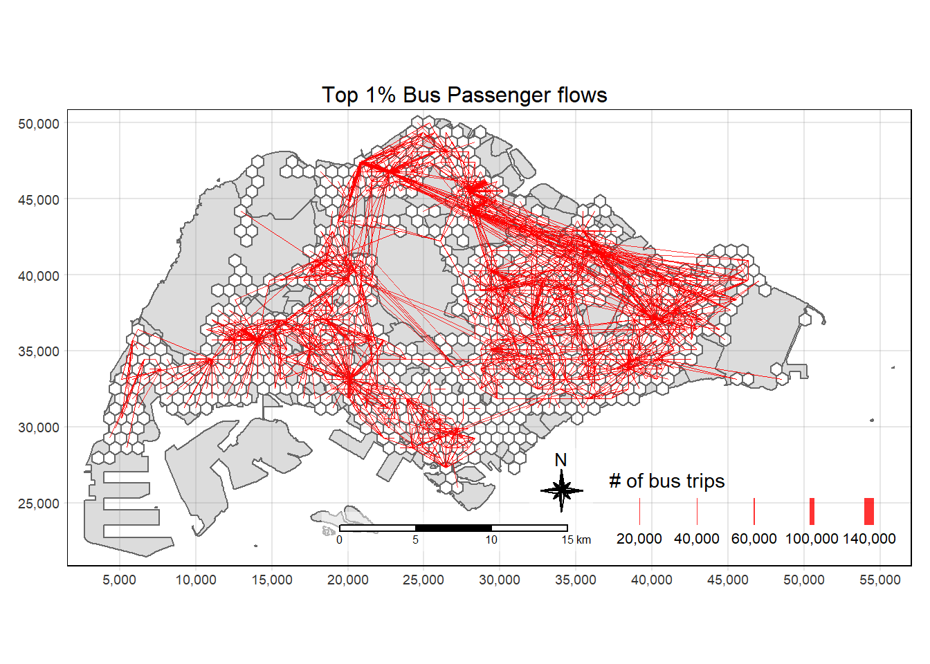

Plotting TRIPS vs DISTANCE

ggplot(SIM_data,
       aes(x = DISTANCE, y = TRIPS)) +
  geom_point() +
  geom_hline(yintercept = 2386, color = "red", linetype = "dashed") +
  annotate("text", x = 20000,
           y = 600, label = "95th percentile",
           hjust = -0.1, color = "red", size = 3) +
  geom_hline(yintercept = 1510, color = "purple", linetype = "dashed") +
  annotate("text", x = 20000,
           y = 1800, label = "99th percentile",
           hjust = -0.1, color = "purple", size = 3) +
  labs(title = "Number of Trips as a Function of Distance",
       x = "Distance (m)",
       y = "Number of Trips")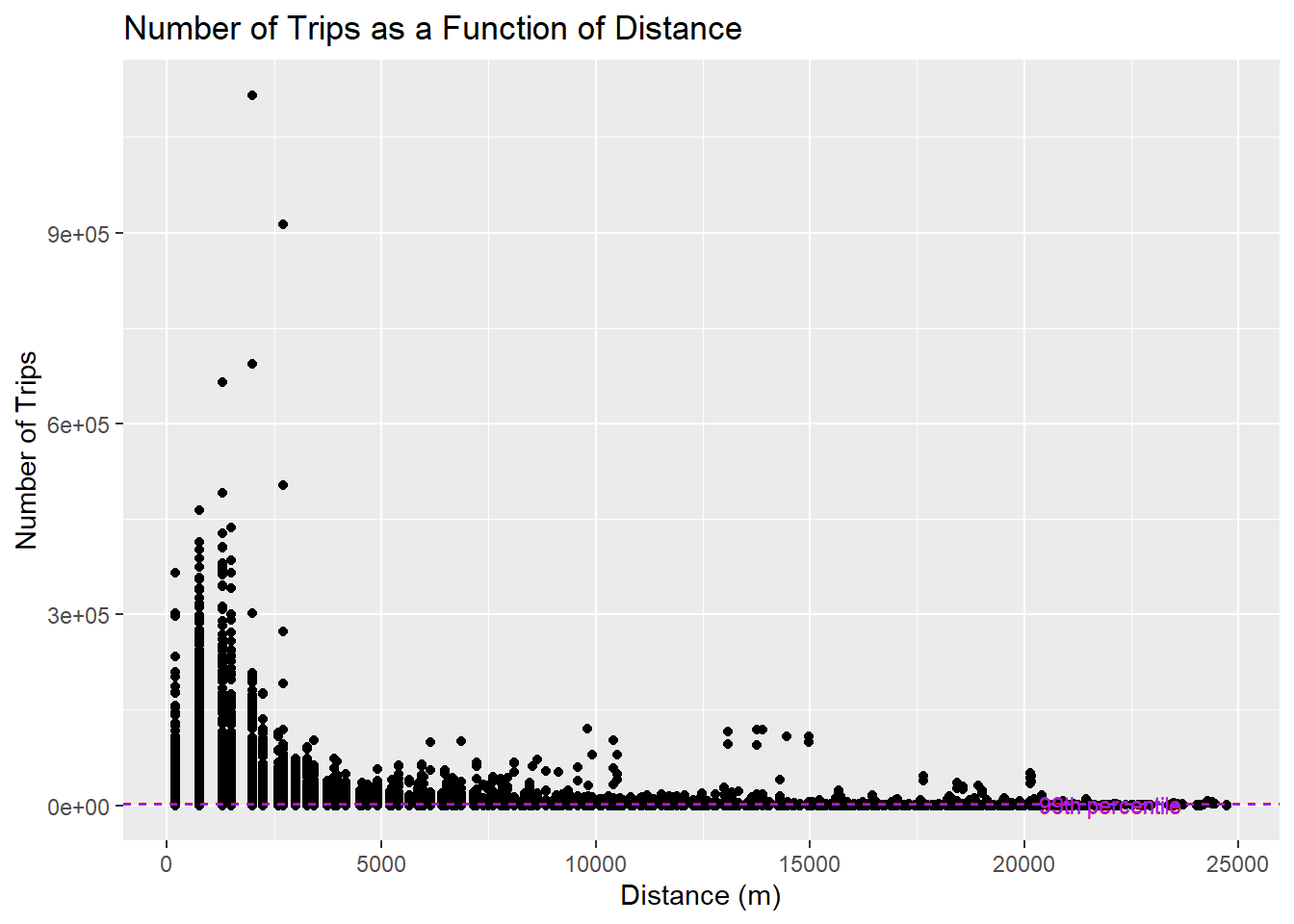

ggplot(SIM_data,
       aes(x = log(DISTANCE), y = log(TRIPS))) +
  geom_point() +
  geom_smooth(method = lm)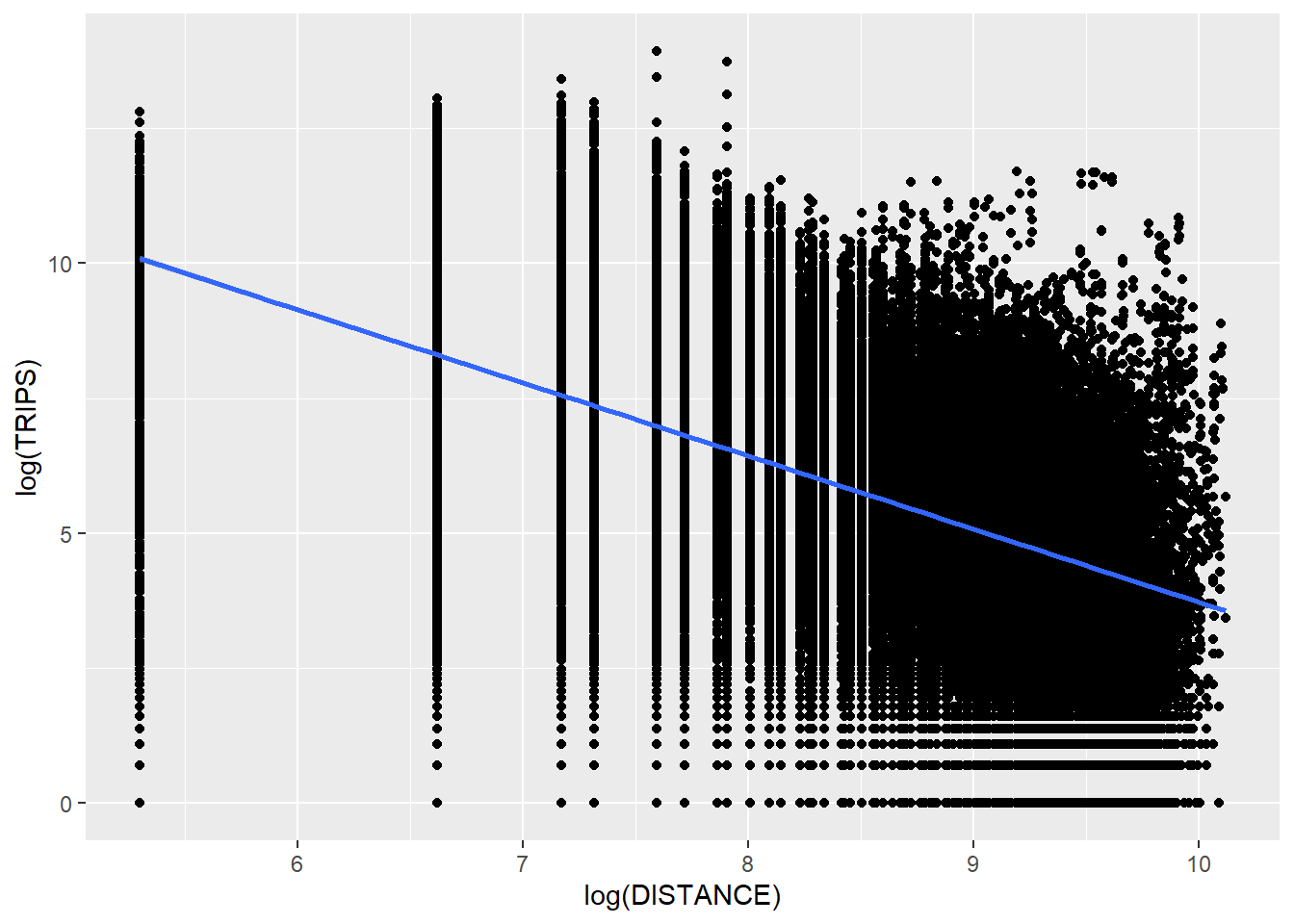

Visualising propulsive forces

::: {callout-tip collapse=“true”} ### Creating a helper function

plot_propulsive <- function(var_name, title_comp, day_type = NULL, hour = NULL, pa=NULL) {
  flowlines_filtered <- flowlines_no_intra
  
  if (!is.null(day_type)) {
    flowlines_filtered <- flowlines_filtered %>% filter(DAY_TYPE == day_type)
  }
  
  if (!is.null(hour)) {
    flowlines_filtered <- flowlines_filtered %>% filter(TIME_PER_HOUR == hour)
  }
  
  if (!is.null(pa)) {
    flowlines_filtered <- flowlines_filtered %>% filter(ORIGIN_SUBZONE == pa)
  }
  
  tm_shape(mpsz3414) +
  tm_polygons("lightgrey", title = "Singapore Boundary") +
  
  # Adding this layer underneath propulsiveness as we removed 0s. from the map
  # so it won't skew the legend
  tm_shape(hex_grids) +
  tm_polygons(col = "white") +
  
  tm_shape(propulsiveness %>% filter(if_any(var_name, ~. >= 1))) +
  tm_polygons(var_name, palette = "Blues", style = "quantile") +
    
  tm_shape(flowlines_no_intra %>% filter(TRIPS > 2385)) +
  tm_lines(lwd = "TRIPS",
           style = "quantile",
           col = "red",
           scale = c(0.1, 1, 3, 5, 7, 10),
           title.lwd = "# of bus trips",
           n = 6,
           alpha = 0.5) +
  
  tm_layout(main.title = paste("Top 1% Bus Passenger Flows and", title_comp),
            main.title.position = "center",
            main.title.size = 1.0,
            legend.height = 0.35, 
            legend.width = 0.35,
            frame = TRUE) +
  
  tm_scale_bar(bg.color = "white", bg.alpha = 0.7, position = c("right", "top")) +
  tm_compass(type="8star", size = 2, bg.color = "white",
             bg.alpha = 0.5, position = c("right", "top")) +
  tm_grid(alpha = 0.2) +
  tm_credits("*Passenger data",
             bg.color = "white", bg.alpha = 0.7,
             position = c("left", "bottom"))
}

:::

Looking at transfers from Buses.

plot_propulsive("BUS_ALIGHT_COUNT", "Potential Transfers from Bus")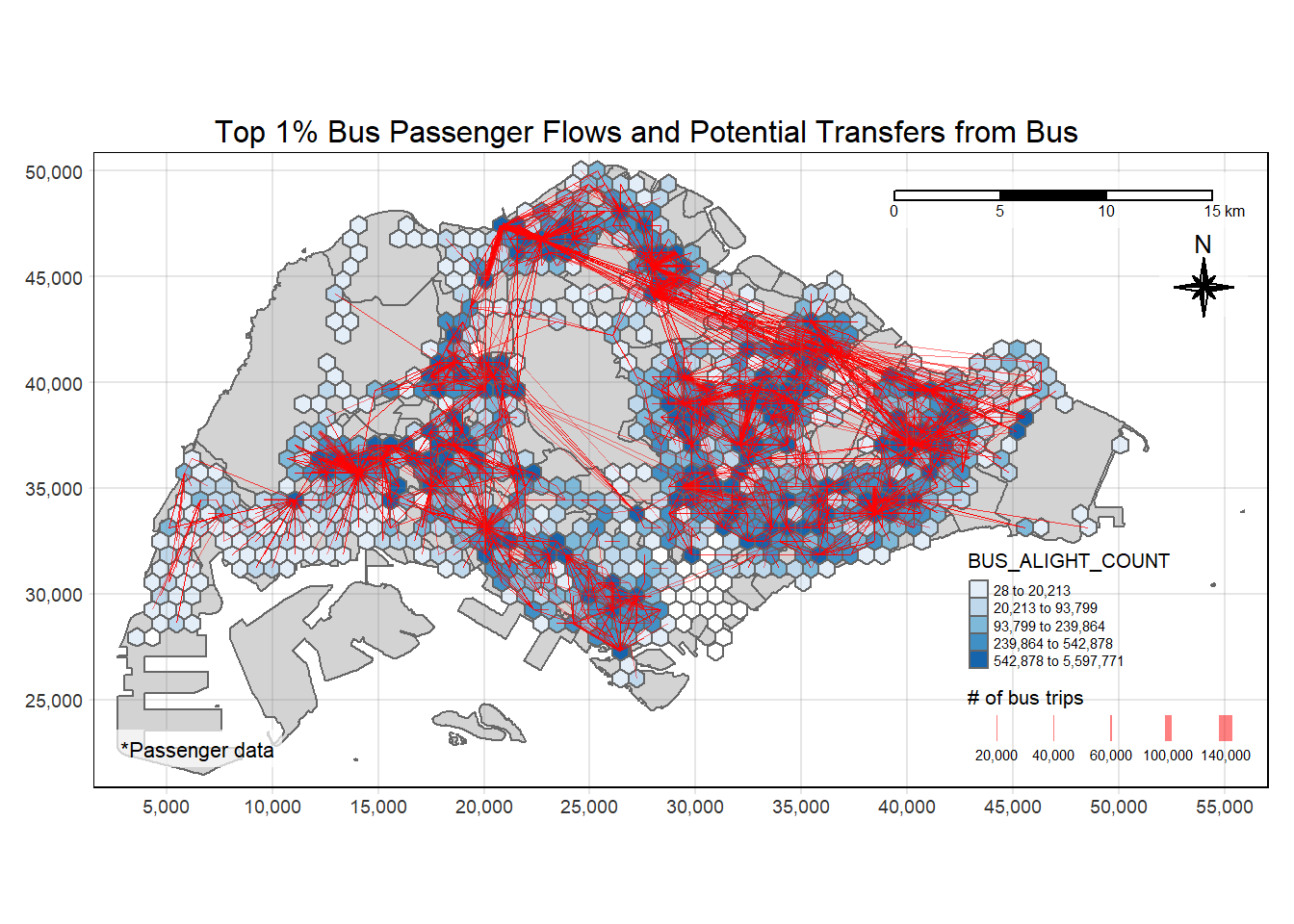

Visualising attractive forces

::: {callout-tip collapse=“true”} ### Creating a helper function

plot_attractive <- function(var_name, title_comp, day_type = NULL, hour = NULL, pa = NULL) {
  flowlines_filtered <- flowlines_no_intra
  
  if (!is.null(day_type)) {
    flowlines_filtered <- flowlines_filtered %>% filter(DAY_TYPE == day_type)
  }
  
  if (!is.null(hour)) {
    flowlines_filtered <- flowlines_filtered %>% filter(TIME_PER_HOUR == hour)
  }
  
  if (!is.null(pa)) {
    flowlines_filtered <- flowlines_filtered %>% filter(DESTINATION_SUBZONE == pa)
  }
  
  tm_shape(mpsz3414) +
  tm_polygons("green", title = "Singapore Boundary") +
  
  # Adding this layer underneath attractiveness as we removed 0s. from the map
  # so it won't skew the legend
  tm_shape(hex_grids) +
  tm_polygons(col = "white") +
  
  tm_shape(attractiveness %>% filter(if_any({{var_name}}, ~. >= 1))) +
  tm_polygons({{var_name}}, palette = "Purples", style = "quantile") +
    
  tm_shape(flowlines_filtered %>% filter(TRIPS > 2385)) +
  tm_lines(lwd = "TRIPS",
           style = "quantile",
           col = "red",
           scale = c(0.1, 1, 3, 5, 7, 10),
           title.lwd = "# of bus trips",
           n = 6,
           alpha = 0.5) +
  
  tm_layout(main.title = paste("Top 1% Bus Passenger Flows and", {{title_comp}}),
            main.title.position = "center",
            main.title.size = 1.0,
            legend.height = 0.35, 
            legend.width = 0.35,
            frame = TRUE) +
  
  tm_scale_bar(bg.color = "white", bg.alpha = 0.7, position = c("right", "top")) +
  tm_compass(type="8star", size = 2, bg.color = "white",
             bg.alpha = 0.5, position = c("right", "top")) +
  tm_grid(alpha = 0.2) +
  tm_credits("*Passenger data",
             bg.color = "white", bg.alpha = 0.7,
             position = c("left", "bottom"))
}

:::

plot_attractive("BUS_STOP_COUNT", "Number of Bus Stops")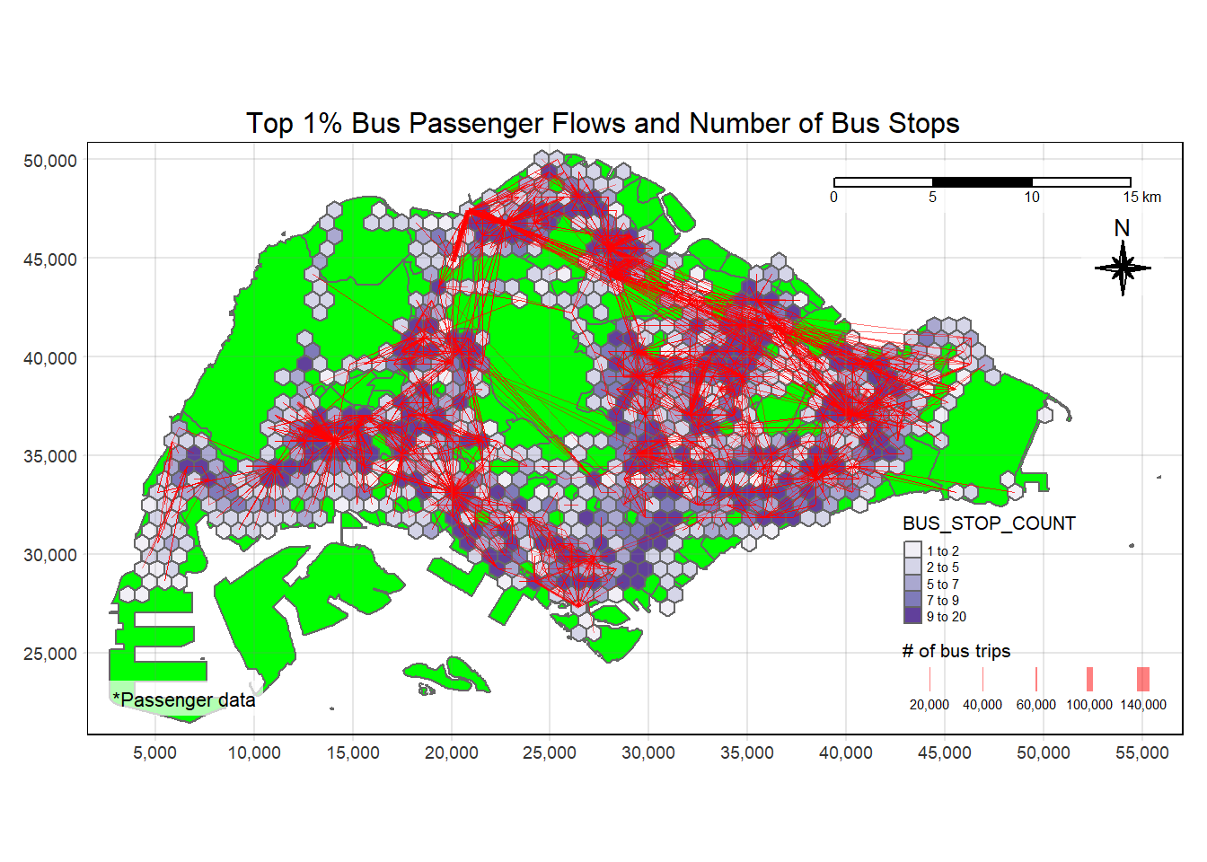

plot_attractive("HDB_COUNT", "Number of HDB Blocks")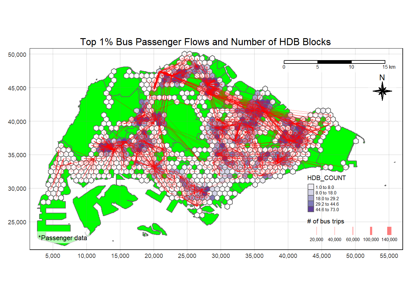

plot_attractive("BIZ_COUNT", "Number of Business Locations", day_type = "WEEKENDS/HOLIDAY")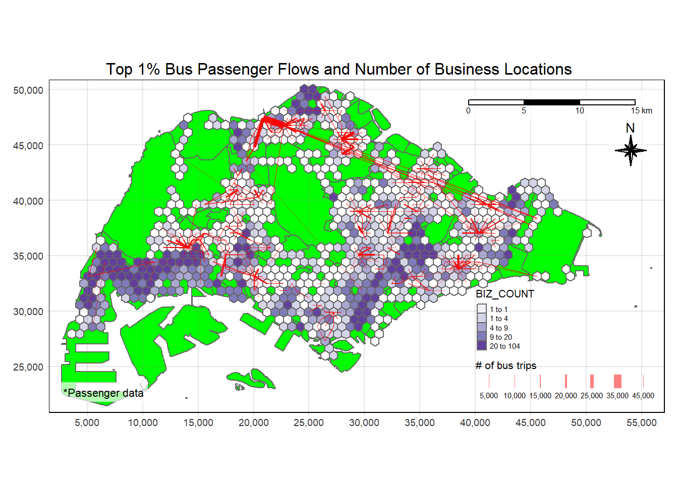

plot_attractive("ENTERTN_COUNT", "Number of Entertainment \nLocations at 5pm on Weekdays", day_type = "WEEKDAY", hour=17)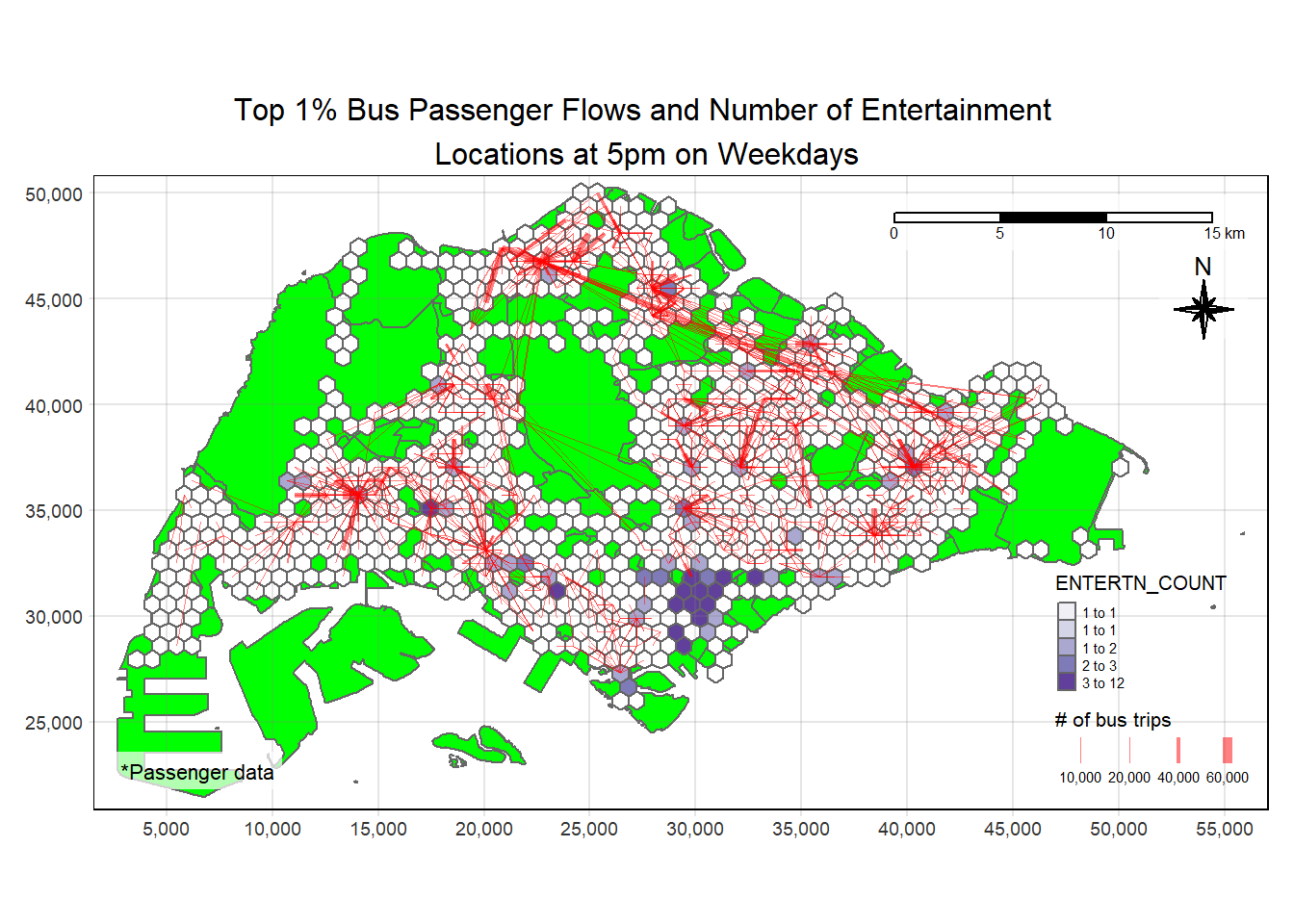

plot_attractive("FOOD_BEV_COUNT", "Number of F&B Locations", pa = "BEDOK")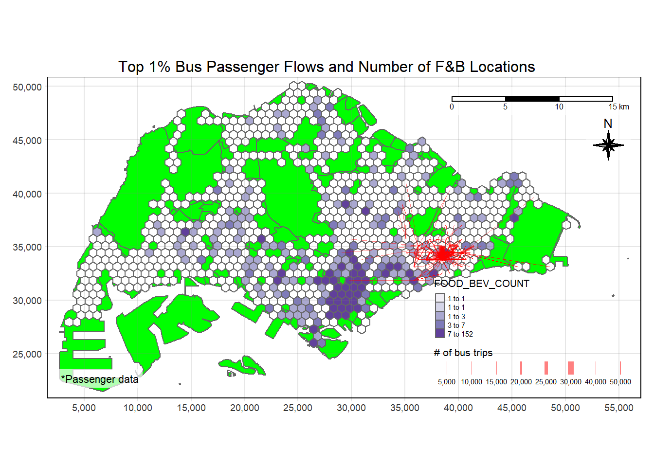

plot_attractive("LEISURE_COUNT", "Number of Leisure \n& Recreation Spots attracting flows to Bedok and Paya Lebar", pa = c("BEDOK", "PAYA LEBAR"))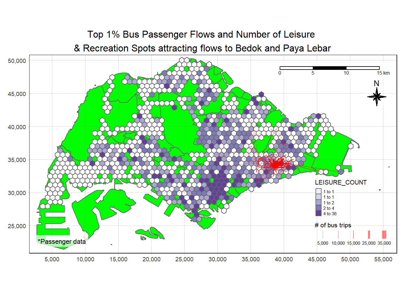

plot_attractive("RETAIL_COUNT", "Number of Retail Locations at 1pm", hour = 13)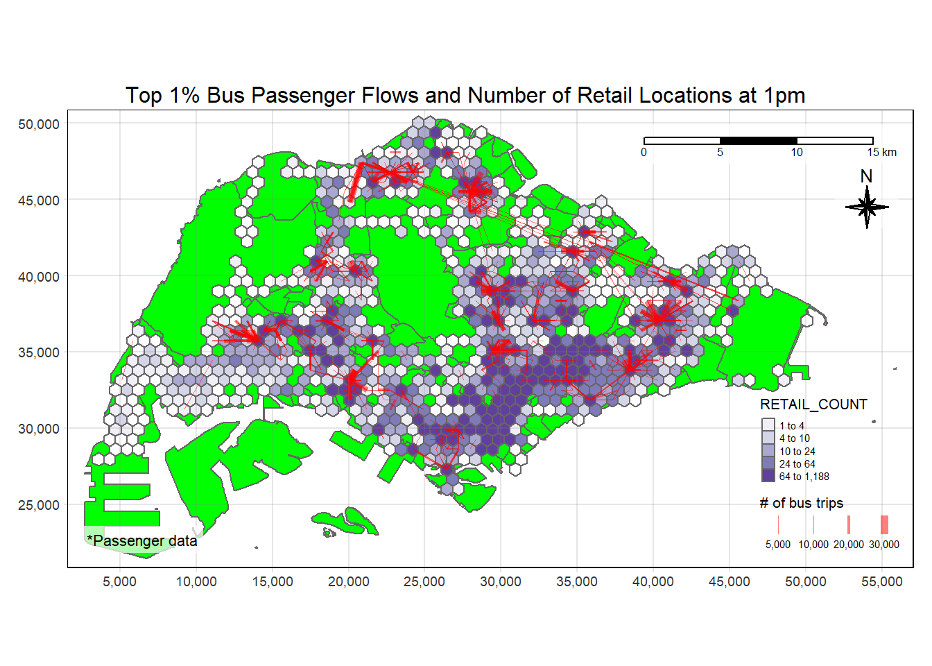

plot_attractive("FIN_COUNT", "Number of Financial Service Locations")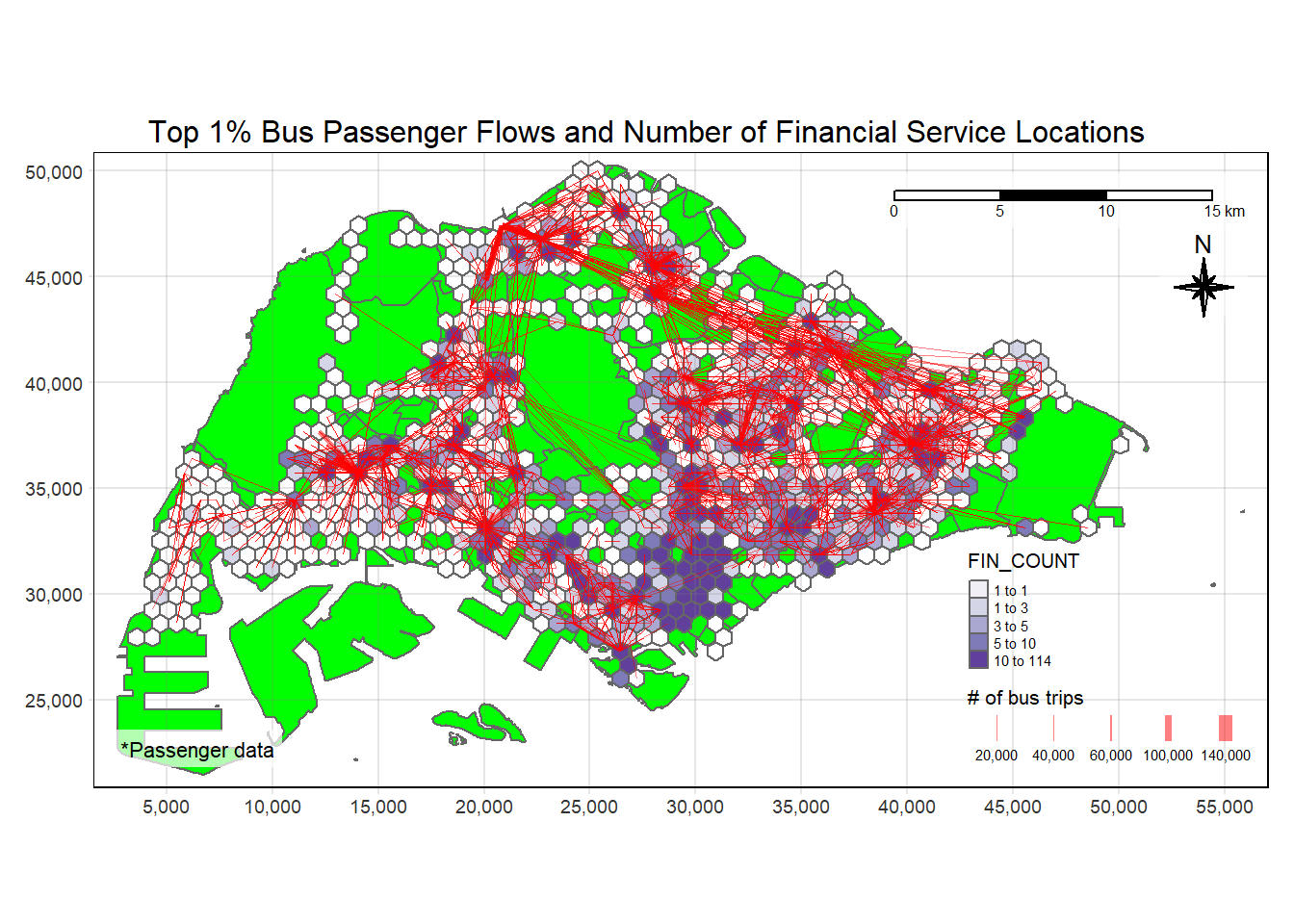

plot_attractive("HC_COUNT", "Number of Public Healthcare Spots")

plot_attractive("SCH_COUNT", "Number of School Locations")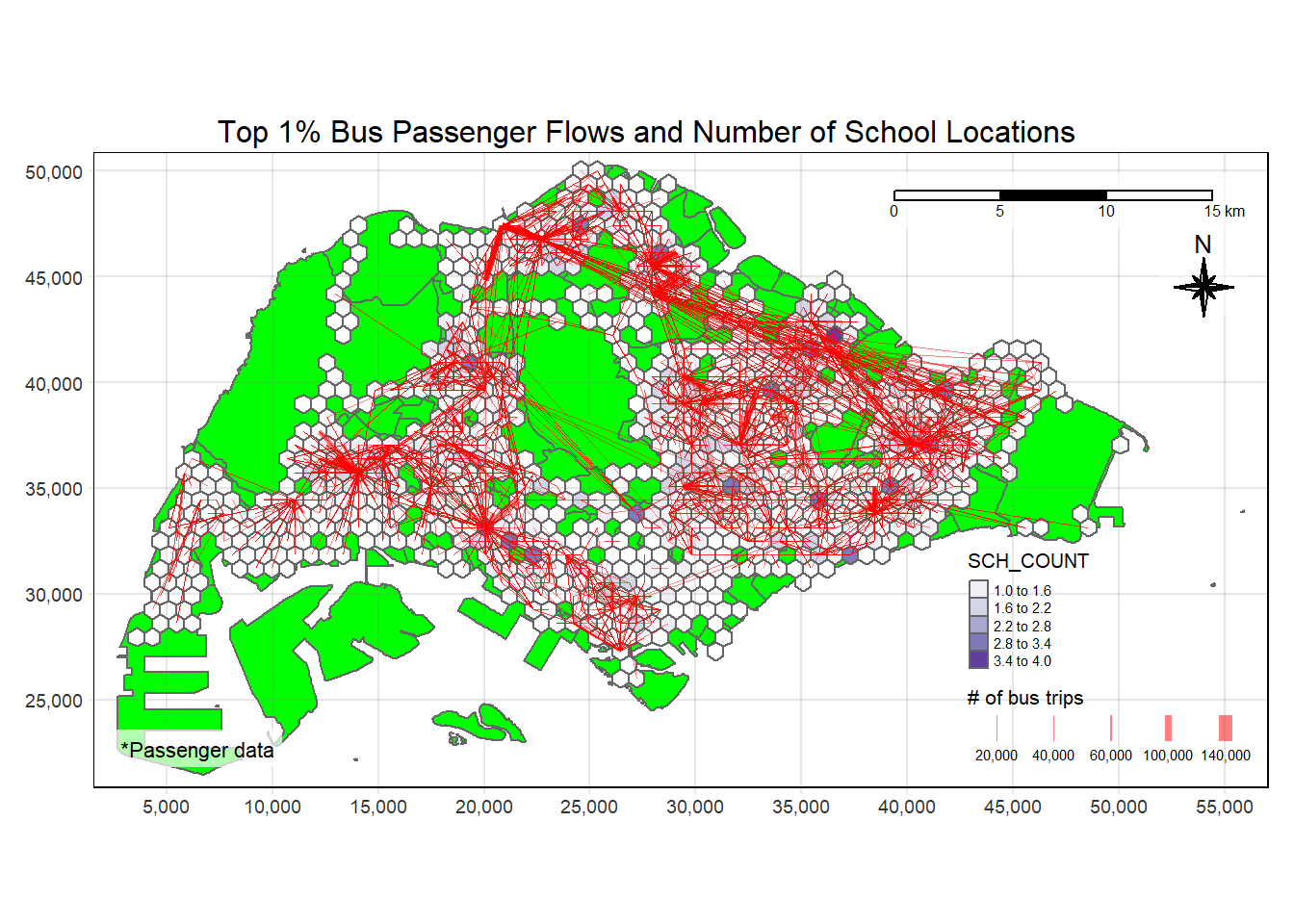

7.1 Prototype Potential

The user inputs will include:

Flow direction with the choices of Overall, Outgoing, Incoming
A viewing level drop-down bar with choices of Overall, PLN_AREA. If PLN_AREA is selected, there will be a further drp-down feature for the user to select the interested planning areas of the Origins and Destinations.
Day type with the choices of Overall, WEEKDAY, WEEKENDS/HOLIDAYS
Time hour choice in a sliding bar style, ranging from 0 to 23.
A sliding bar to control the number of trips shown based on the user inputs

8.0 Spatial Econometric Interaction Modelling

Remove the intra-zonal zones pairs from SIM_data.

SIM_data_no_intra <- SIM_data %>% filter(ORIG_HEX_ID != DEST_HEX_ID)

To calibrate SEIM using spflow package, three data sets are required:

Spatial Weights
Distance Matrix
Explanatory Variables

Prepare Spatial Weights

hex_grid <- st_make_grid(mpsz3414, cellsize = c(750, 750), what = "polygons", square = FALSE) %>%
  st_sf() %>%
  # Apply as.factor() since index will be used as the identifier to link to other data sets
  mutate(index = as.factor(row_number()))

# Create border of Singapore's land area
mpsz_border <- mpsz3414 %>% st_union()

# Clip the hexagon grid layer
hex_grid_bounded <- st_intersection(hex_grid, mpsz_border)

# Check if hex grid intersects any polygons using st_intersects
# Returns a list of intersecting hexagons
intersection_list = hex_grid$index[lengths(st_intersects(hex_grid, hex_grid_bounded)) > 0]

# Filter for the intersecting hexagons
hex_grids = hex_grid %>%
  filter(index %in% intersection_list)


hex_grids$BUS_COUNT <- lengths(st_intersects(hex_grids, BusStop))
hex_grids$ENTERTN_COUNT <- lengths(st_intersects(hex_grids, entertn))
hex_grids$FOOD_BEV_COUNT <- lengths(st_intersects(hex_grids, food_bev))
hex_grids$LEISURE_COUNT <- lengths(st_intersects(hex_grids, leis_rec))
hex_grids$RETAIL_COUNT <- lengths(st_intersects(hex_grids, retail))
hex_grids$BIZ_COUNT <- lengths(st_intersects(hex_grids, biz))
hex_grids$FIN_COUNT <- lengths(st_intersects(hex_grids, fin))
hex_grids$HDB_COUNT <- lengths(st_intersects(hex_grids, hdb_residential2))
hex_grids$HC_COUNT <- lengths(st_intersects(hex_grids, hc))
hex_grids$SCHOOL_COUNT <- lengths(st_intersects(hex_grids, schools))


tm_shape(hex_grids) +
  tm_fill(col = "BUS_COUNT",
          palette = "Blues",
          style = "cont",
          title = "Bus Stop Density") +
  tm_borders(col="grey")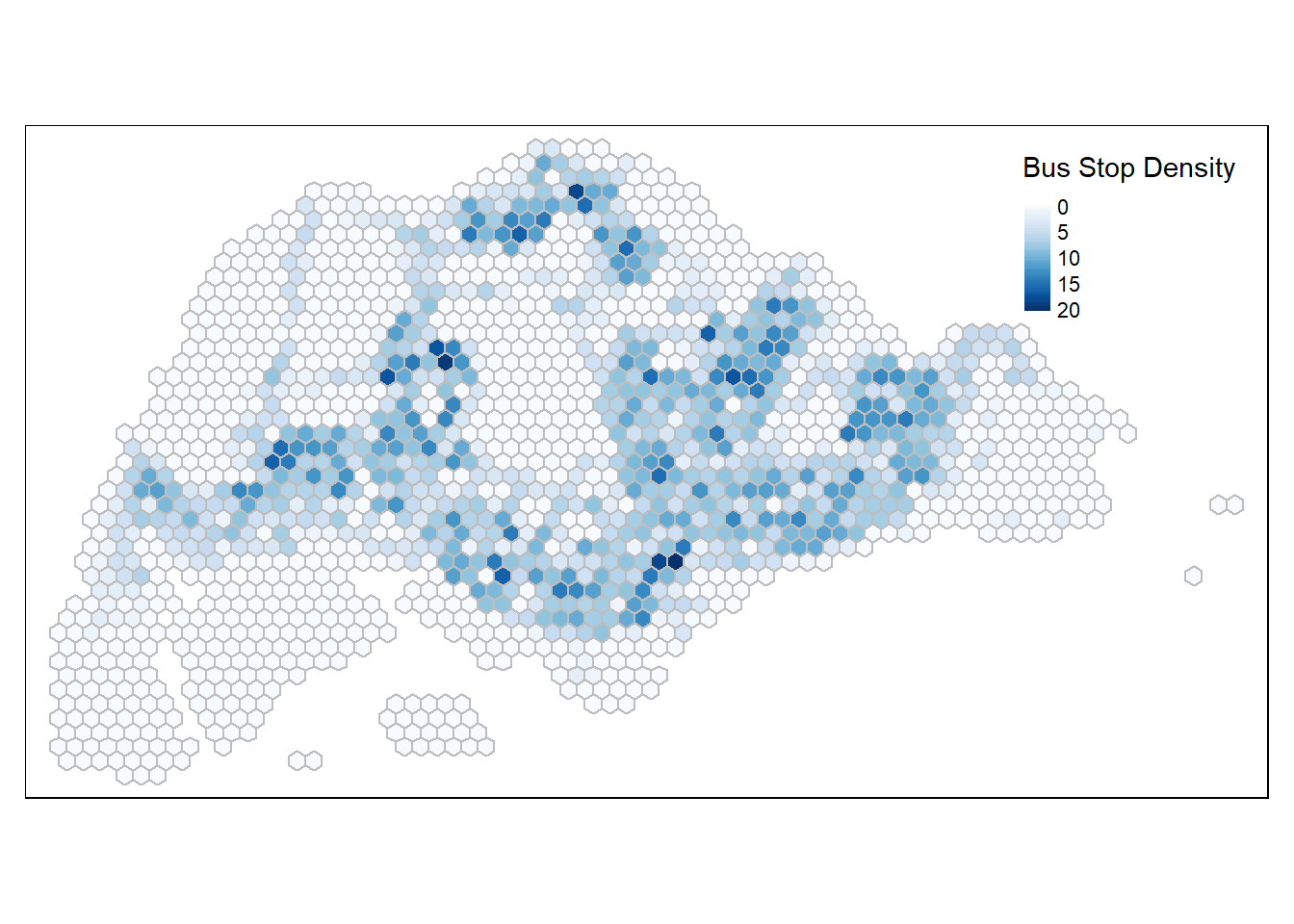

coords <- hex_grids %>%
  filter("BUS_COUNT" > 0) %>%
  select(geometry) %>%
  st_centroid()

k1 <- knn2nb(knearneigh(coords))
k1dists <- unlist(nbdists(k1, coords, longlat = FALSE))

# Print summary report
summary(k1dists)

   Min. 1st Qu.  Median    Mean 3rd Qu.    Max. 
  750.0   750.0   750.0   751.6   750.0  3436.9

The largest first nearest neighbour distance is 2461.2.

centroids <- suppressWarnings({
    st_point_on_surface(st_geometry(hex_grids))})

hexgrid_nb <- list(
  "by_contiguity" = poly2nb(hex_grids),
  "by_distance" = dnearneigh(centroids, 
                             d1 = 0, d2 = 3437),
  "by_knn" = knn2nb(knearneigh(centroids, 6))
)

hexgrid_nb

$by_contiguity
Neighbour list object:
Number of regions: 1673 
Number of nonzero links: 9478 
Percentage nonzero weights: 0.3386295 
Average number of links: 5.665272 
1 region with no links:
1671
5 disjoint connected subgraphs

$by_distance
Neighbour list object:
Number of regions: 1673 
Number of nonzero links: 119676 
Percentage nonzero weights: 4.275778 
Average number of links: 71.53377 
2 disjoint connected subgraphs

$by_knn
Neighbour list object:
Number of regions: 1673 
Number of nonzero links: 10038 
Percentage nonzero weights: 0.3586372 
Average number of links: 6 
2 disjoint connected subgraphs
Non-symmetric neighbours list

Preparing Flow Data

flowlines$DISTANCE <- dist_tbl$DISTANCE[match(paste(flowlines$ORIG_HEX_ID, flowlines$DEST_HEX_ID), paste(dist_tbl$ORIG_HEX_ID, dist_tbl$DEST_HEX_ID))]

flow_data <- flowlines %>%
  select(ORIG_HEX_ID, DEST_HEX_ID, TRIPS, DISTANCE) %>%
  group_by(ORIG_HEX_ID, DEST_HEX_ID, DISTANCE) %>%
  summarise(TRIPS = sum(TRIPS)) %>%
  ungroup()

write_rds(flow_data, "data/rds/flow_data_3b.rds")

flow_data <- read_rds("data/rds/flow_data_3b.rds")

Preparing Explanatory Variables

explanatory <- hex_grids %>%
  st_drop_geometry()

write_rds(explanatory, "data/rds/explanatory.rds")

explanatory <- read_rds("data/rds/explanatory.rds")

Creating spflow_network-class objects

hex_net <- spflow_network(
  id_net = "sg",  # assign an id name, can give it any input
  node_neighborhood = nb2mat(hexgrid_nb$by_distance),
  node_data = explanatory,
  node_key_column = "index"
)

hex_net

Spatial network nodes with id: sg
--------------------------------------------------
Number of nodes: 1673
Average number of links per node: 71.534
Density of the neighborhood matrix: 4.28% (non-zero connections)

Data on nodes:
     index BUS_COUNT ENTERTN_COUNT FOOD_BEV_COUNT LEISURE_COUNT RETAIL_COUNT
1       25         0             0              0             0            0
2       26         0             0              0             0            0
3       27         0             0              0             0            0
4       28         0             0              0             0            0
5       29         0             0              0             0            0
6       47         0             0              0             0            0
---    ---       ---           ---            ---           ---          ---
1668  2957         0             0              0             0            0
1669  3003         0             0              0             0            0
1670  3026         0             0              0             0            0
1671  3205         0             0              0             0            0
1672  3276         0             0              0             0            0
1673  3322         0             0              0             0            0
     BIZ_COUNT FIN_COUNT HDB_COUNT HC_COUNT SCHOOL_COUNT
1            0         0         0        0            0
2            0         0         0        0            0
3            0         0         0        0            0
4            0         0         0        0            0
5            0         0         0        0            0
6            0         0         0        0            0
---        ---       ---       ---      ---          ---
1668         0         0         0        0            0
1669         0         0         0        0            0
1670         0         0         0        0            0
1671         0         0         0        0            0
1672         0         0         0        0            0
1673         0         0         0        0            0

Create spflow_network_pair-class using spflow_network_pair()

hex_net_pairs <- spflow_network_pair(
  id_orig_net = "sg",
  id_dest_net = "sg",
  pair_data = flow_data,
  orig_key_column = "ORIG_HEX_ID",
  dest_key_column = "DEST_HEX_ID"
)

hex_net_pairs

hex_multi_net <- spflow_network_multi(hex_net, hex_net_pairs)

hex_multi_net

References

M. Chan. Applied Spatial Interaction Models - Case Study of Singapore Public Bus Commuter Flows. https://geospatial2023.netlify.app/take_home_exercise/ex2/take_home_ex2#calibrate-spatial-econometric-interaction-model-usng-maximum-likelihood-estimation

K. J. Paas, 2023. Take Home Exercise 2: A Case Study of Singapore Public Bus Commuter Flows. https://isss624-kjcpaas.netlify.app/take-home_ex2/take-home_ex2

T. S. Kam.