In-class Exercise 5

Installing and Loading Packages

• sfdep creates a sf and tidyverse friendly interface to the package.

pacman::p_load(sf, tmap, sfdep, tidyverse, dplyr)

Data

The two data sets we will use are: - Hunan, a geospatial data in ESRI shape file format - Hunan_2012, aspatial attribute data in csv format

Import geospatial data

hunan <- st_read(dsn="data/geospatial", layer="Hunan")

Reading layer `Hunan' from data source 
  `C:\guacodemoleh\IS415-GAA\In-class_Ex\In-class_Ex05\data\geospatial' 
  using driver `ESRI Shapefile'
Simple feature collection with 88 features and 7 fields
Geometry type: POLYGON
Dimension:     XY
Bounding box:  xmin: 108.7831 ymin: 24.6342 xmax: 114.2544 ymax: 30.12812
Geodetic CRS:  WGS 84

Importing aspatial data

hunan2012 <- read_csv("data/aspatial/Hunan_2012.csv")

Combining aspatial fields to geospatial data

hunan_GDPPC <- left_join(hunan,hunan2012) %>%
  select(1:4, 7, 15)

Plotting Choropleth Map

tmap_mode("plot")
tm_shape(hunan_GDPPC) +
  tm_fill(col="GDPPC",
          style = "quantile",
          palette = "Blues",
          title = "GDPPC") +
  tm_layout(main.title = "Distribution of GDP per capita by County",
            main.title.position = "center",
            main.title.size =1.2,
            legend.height = 0.45,
            legend.width = 0.35,
            frame = TRUE) +
  tm_borders(alpha = 0.5) +
  tm_compass(type="8star", size = 2) +
  tm_scale_bar() +
  tm_grid(alpha = 0.2)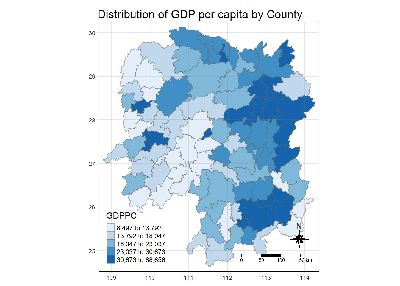

Global Measures of Spatial Association

The queen method is used to derive the contiguity weights

wm_q <- hunan_GDPPC %>%
  mutate(nb = st_contiguity(geometry),
         wt = st_weights(nb,
                         style = "W"),
         .before = 1)

Computing Global Moran’s I

moranI <- global_moran(wm_q$GDPPC,
                       wm_q$nb,
                       wm_q$wt)
glimpse(moranI)

List of 2
 $ I: num 0.301
 $ K: num 7.64

global_moran_test(wm_q$GDPPC,
                       wm_q$nb,
                       wm_q$wt)

    Moran I test under randomisation

data:  x  
weights: listw    

Moran I statistic standard deviate = 4.7351, p-value = 1.095e-06
alternative hypothesis: greater
sample estimates:
Moran I statistic       Expectation          Variance 
      0.300749970      -0.011494253       0.004348351 

Performing Global Moran’s I permutation test

It is better to conduct permutation tests.

set.seed(1234)

global_moran_perm(wm_q$GDPPC,
                  wm_q$nb,
                  wm_q$wt,
                  nsim = 99) 

    Monte-Carlo simulation of Moran I

data:  x 
weights: listw  
number of simulations + 1: 100 

statistic = 0.30075, observed rank = 100, p-value < 2.2e-16
alternative hypothesis: two.sided

• nsim refers to the number of simulations
• Since the p-value is < 0.05, there is sufficient evidence to reject the null hypothesis that the spatial distribution of GDP per capita resembles a random distribution, or rather the distribution is independent from spatial. Since Moran’s I statistic is > 0, we can infer that the spatial distribution shows signs of clustering.