pacman::p_load(tmap, sf, sp, performance, reshape2, ggpubr, tidyverse, stplanr, knitr)Takehome-Ex 3: Exploratory Spatial Data Analysis for Potential Push & Pull Factors of Locations in Singapore using Public Bus Data
Overview
In this exercise, my focus would be on prototyping exploratory spatial data analysis, particularly density of spatial assets within hexagonal traffic analysis zones. In conventional geography, a traffic analysis zone is the unit most commonly used in transportation planning models and the size of it varies. Hexagonal traffic analysis zones has gained traction as the hexagons of the study area have a uniform size which are easily comparable with each other when determining transport attractiveness. It is also recommended that hexagon radius should be 125m for areas in high urbanisation and 250m in areas with less urbanisation (Chmielewski et al., 2020).
Package Installation
Data Preparation
URA’s Masterplan Subzone 2019 Layer in shapefile format
Bus Stop Locations extracted from LTA
A tabulated bus passenger flow for Nov 2023, Dec 2023 and Jan 2024 from LTA dynamic data mall
Population Data for 2023 from SingStat
Schools from MOE
Financial Services
Hospitals, polyclinics and CHAS clinics derived from Google Maps
Subzone Layer
Read the subzone layer
mpsz <- st_read("data/geospatial/master-plan-2019-subzone-boundary-no-sea-kml.kml")Reading layer `URA_MP19_SUBZONE_NO_SEA_PL' from data source
`C:\guacodemoleh\IS415-GAA\Take-home_Ex\Take-home_Ex03\data\geospatial\master-plan-2019-subzone-boundary-no-sea-kml.kml'
using driver `KML'
Simple feature collection with 332 features and 2 fields
Geometry type: MULTIPOLYGON
Dimension: XY, XYZ
Bounding box: xmin: 103.6057 ymin: 1.158699 xmax: 104.0885 ymax: 1.470775
z_range: zmin: 0 zmax: 0
Geodetic CRS: WGS 84Convert mpsz to 2D geometry.
mpsz <- st_zm(mpsz, drop = TRUE) # Convert 3D geometries to 2DExtract the SUBZONE_N and PLN_AREA_N from the Dscrptn field
For SUBZONE_N,
mpsz <- mpsz %>%
  rowwise() %>%
  mutate(SUBZONE_N = str_extract(Description, "<th>SUBZONE_N</th> <td>(.*?)</td>")) %>%
  ungroup()

mpsz$SUBZONE_N <- str_remove_all(mpsz$SUBZONE_N, "<.*?>|SUBZONE_N")
For PLN_AREA_N,
mpsz <- mpsz %>%
  rowwise() %>%
  mutate(PLN_AREA_N = str_extract(Description, "<th>PLN_AREA_N</th> <td>(.*?)</td>")) %>%
  ungroup()

mpsz$PLN_AREA_N <- str_remove_all(mpsz$PLN_AREA_N, "<.*?>|PLN_AREA_N")
Remove the Description column
mpsz$Description <- NULLCreate the shapefile
st_write(mpsz, "data/geospatial/mpsz_sf.shp")Read the updated shapefile.
mpsz_sf <- st_read("data/geospatial/mpsz_sf.shp")Reading layer `mpsz_sf' from data source
`C:\guacodemoleh\IS415-GAA\Take-home_Ex\Take-home_Ex03\data\geospatial\mpsz_sf.shp'
using driver `ESRI Shapefile'
Simple feature collection with 332 features and 3 fields
Geometry type: MULTIPOLYGON
Dimension: XY
Bounding box: xmin: 103.6057 ymin: 1.158699 xmax: 104.0885 ymax: 1.470775
Geodetic CRS: WGS 84mpsz_sp <- as(mpsz_sf, "Spatial")Creating Spatial Grids
mpsz3414 <- st_transform(mpsz_sf, 3414)
outer_islands <- c("SEMAKAU", "SUDONG", "NORTH-EASTERN ISLANDS", "SOUTHERN GROUP")
mpsz3414 <- mpsz3414 %>%
  filter(!str_trim(SUBZONE_N) %in% str_trim(outer_islands))
hex_grid <- st_make_grid(mpsz3414, cellsize = c(750, 750), what = "polygons", square = FALSE) %>%
st_sf() %>%
# Apply as.factor() since index will be used as the identifier to link to other data sets
mutate(index = as.factor(row_number()))
# Create border of Singapore's land area
mpsz_border <- mpsz3414 %>% st_union()
# Clip the hexagon grid layer
hex_grid_bounded <- st_intersection(hex_grid, mpsz_border)tmap_mode("plot")
tm_shape(hex_grid_bounded) +
tm_polygons()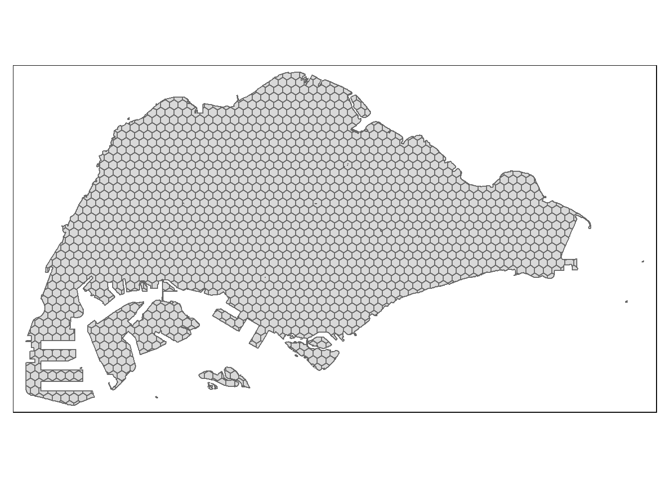
# Check if hex grid intersects any polygons using st_intersects
# Returns a list of intersecting hexagons
intersection_list = hex_grid$index[lengths(st_intersects(hex_grid, hex_grid_bounded)) > 0]

# Filter for the intersecting hexagons
hex_grid_bounded2 = hex_grid %>%
  filter(index %in% intersection_list)

tm_shape(hex_grid_bounded2) +
  tm_polygons()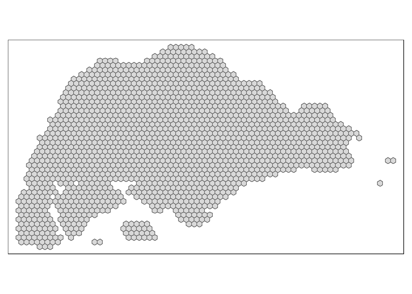
- The map above now shows the complete analytical hexagon data of 375m (perpendicular distance between the centre of hexagon and its edges) that represents the TAZ.
Bus Stop Locations
BusStop <- read.csv("data/aspatial/bus_coords_subzone.csv") %>% st_as_sf(coords=c("Longitude", "Latitude"), crs=4326) %>%
  st_transform(crs=3414)
Compute Bus Stop Density
Using st_intersects(), we can intersect the bus stops layer and the hexagon layer and use lengths() to count the number of bus stops that lie inside each Traffic Analysis Zone. These count values are appended back to each spatial grid and encapsulated into a new column called busstop_count in a duplicated dataframe, hex_grid_bounded2.
hex_grid_bounded2$busstop_count <- lengths(st_intersects(hex_grid_bounded2, BusStop))tm_shape(hex_grid_bounded2) +
tm_fill(col = "busstop_count",
palette = "Blues",
style = "cont",
title = "Bus Stop Density") +
tm_borders(col = "grey") +
tm_legend(position = c("RIGHT", "BOTTOM"))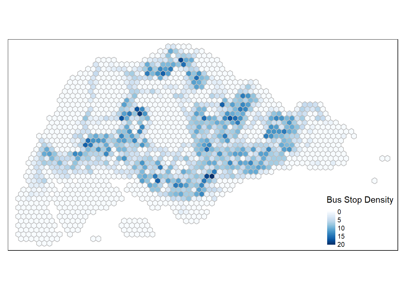
write_rds(hex_grid_bounded2, "data/rds/hex_grid_bounded2")hex_grid_bounded2 <- readRDS("data/rds/hex_grid_bounded2")Constructing O-D Matrix of commuter flow
od_bus_nov <- read_csv("data/OD Bus/origin_destination_bus_202311.csv")
od_bus_dec <- read_csv("data/OD Bus/origin_destination_bus_202312.csv")
od_bus_jan <- read_csv("data/OD Bus/origin_destination_bus_202401.csv")
OD <- rbind(od_bus_nov, od_bus_dec)
OD <- rbind(OD, od_bus_jan)
nrow(od_bus_nov) + nrow(od_bus_dec) + nrow(od_bus_jan) == nrow(OD)[1] TRUEstr(OD)spc_tbl_ [12,316,954 × 7] (S3: spec_tbl_df/tbl_df/tbl/data.frame)
$ YEAR_MONTH : chr [1:12316954] "2023-11" "2023-11" "2023-11" "2023-11" ...
$ DAY_TYPE : chr [1:12316954] "WEEKENDS/HOLIDAY" "WEEKDAY" "WEEKENDS/HOLIDAY" "WEEKDAY" ...
$ TIME_PER_HOUR : num [1:12316954] 16 16 14 14 17 17 17 7 7 14 ...
$ PT_TYPE : chr [1:12316954] "BUS" "BUS" "BUS" "BUS" ...
$ ORIGIN_PT_CODE : chr [1:12316954] "04168" "04168" "80119" "80119" ...
$ DESTINATION_PT_CODE: chr [1:12316954] "10051" "10051" "90079" "90079" ...
$ TOTAL_TRIPS : num [1:12316954] 6 4 4 8 2 18 1 1 2 3 ...
- attr(*, "spec")=
.. cols(
.. YEAR_MONTH = col_character(),
.. DAY_TYPE = col_character(),
.. TIME_PER_HOUR = col_double(),
.. PT_TYPE = col_character(),
.. ORIGIN_PT_CODE = col_character(),
.. DESTINATION_PT_CODE = col_character(),
.. TOTAL_TRIPS = col_double()
.. )
- attr(*, "problems")=<externalptr> ORIGIN_PT_CODE and DESTINATION_PT_CODE are listed as character variables. These variables should be transformed to factors so that R treats them as grouping variables.
cols_to_convert <- c("ORIGIN_PT_CODE", "DESTINATION_PT_CODE")

OD[cols_to_convert] <- lapply(OD[cols_to_convert], as.factor)

glimpse(OD)
Rows: 12,316,954
Columns: 7
$ YEAR_MONTH <chr> "2023-11", "2023-11", "2023-11", "2023-11", "2023-…
$ DAY_TYPE <chr> "WEEKENDS/HOLIDAY", "WEEKDAY", "WEEKENDS/HOLIDAY",…
$ TIME_PER_HOUR <dbl> 16, 16, 14, 14, 17, 17, 17, 7, 7, 14, 14, 10, 10, …
$ PT_TYPE <chr> "BUS", "BUS", "BUS", "BUS", "BUS", "BUS", "BUS", "…
$ ORIGIN_PT_CODE <fct> 04168, 04168, 80119, 80119, 44069, 20281, 20281, 1…
$ DESTINATION_PT_CODE <fct> 10051, 10051, 90079, 90079, 17229, 20141, 20141, 1…
$ TOTAL_TRIPS <dbl> 6, 4, 4, 8, 2, 18, 1, 1, 2, 3, 8, 3, 1, 5, 2, 1, 1…ORIGIN_PT_CODEandDESTINATION_PT_CODE` are now factors.
write_rds(OD, "data/rds/odbus_combined.rds")odbus_combined <- readRDS("data/rds/odbus_combined.rds")Commuting Flow Data
Weekday
Morning
od_wkday_morn <- odbus_combined %>%
  filter(DAY_TYPE == "WEEKDAY" & TIME_PER_HOUR >= 6 & TIME_PER_HOUR <= 9) %>%
  group_by(ORIGIN_PT_CODE, DESTINATION_PT_CODE) %>%
  summarise(TRIPS = sum(TOTAL_TRIPS)) %>%
ungroup()head(od_wkday_morn, 10)# A tibble: 10 × 3
ORIGIN_PT_CODE DESTINATION_PT_CODE TRIPS
<fct> <fct> <dbl>
1 01012 01112 469
2 01012 01113 299
3 01012 01121 168
4 01012 01211 244
5 01012 01311 383
6 01012 07371 31
7 01012 60011 49
8 01012 60021 29
9 01012 60031 48
10 01012 60159 41od_wkday_morn_nov <- odbus_combined %>%
filter(DAY_TYPE == "WEEKDAY" & TIME_PER_HOUR >= 6 & TIME_PER_HOUR <= 9 & YEAR_MONTH == "2023-11") %>%
group_by(ORIGIN_PT_CODE, DESTINATION_PT_CODE) %>%
summarise(TRIPS = sum(TOTAL_TRIPS)) %>%
ungroup()od_wkday_morn_dec <- odbus_combined %>%
filter(DAY_TYPE == "WEEKDAY" & TIME_PER_HOUR >= 6 & TIME_PER_HOUR <= 9 & YEAR_MONTH == "2023-12") %>%
group_by(ORIGIN_PT_CODE, DESTINATION_PT_CODE) %>%
summarise(TRIPS = sum(TOTAL_TRIPS)) %>%
ungroup()od_wkday_morn_jan <- odbus_combined %>%
filter(DAY_TYPE == "WEEKDAY" & TIME_PER_HOUR >= 6 & TIME_PER_HOUR <= 9 & YEAR_MONTH == "2024-01") %>%
group_by(ORIGIN_PT_CODE, DESTINATION_PT_CODE) %>%
summarise(TRIPS = sum(TOTAL_TRIPS)) %>%
ungroup()Evening
od_wkday_eve <- odbus_combined %>%
  filter(DAY_TYPE == "WEEKDAY" & TIME_PER_HOUR >= 17 & TIME_PER_HOUR <=20) %>%
  group_by(ORIGIN_PT_CODE, DESTINATION_PT_CODE) %>%
  summarise(TRIPS = sum(TOTAL_TRIPS)) %>%
ungroup()od_wkday_eve_nov <- odbus_combined %>%
filter(DAY_TYPE == "WEEKDAY" & TIME_PER_HOUR >= 17 & TIME_PER_HOUR <= 20 & YEAR_MONTH == "2023-11") %>%
group_by(ORIGIN_PT_CODE, DESTINATION_PT_CODE) %>%
summarise(TRIPS = sum(TOTAL_TRIPS)) %>%
ungroup()od_wkday_eve_dec <- odbus_combined %>%
filter(DAY_TYPE == "WEEKDAY" & TIME_PER_HOUR >= 17 & TIME_PER_HOUR <= 20 & YEAR_MONTH == "2023-12") %>%
group_by(ORIGIN_PT_CODE, DESTINATION_PT_CODE) %>%
summarise(TRIPS = sum(TOTAL_TRIPS)) %>%
ungroup()od_wkday_eve_jan <- odbus_combined %>%
filter(DAY_TYPE == "WEEKDAY" & TIME_PER_HOUR >= 17 & TIME_PER_HOUR <= 20 & YEAR_MONTH == "2024-01") %>%
group_by(ORIGIN_PT_CODE, DESTINATION_PT_CODE) %>%
summarise(TRIPS = sum(TOTAL_TRIPS)) %>%
ungroup()Geospatial Data Wrangling
Now we need to convert the od data from aspatial to geospatial data.
First, we populate the hexagon grid indexes of hex_grid_bounded2 sf data frame into BusStop sf data frame using st_intersection().
BusStop_hex <- st_intersection(BusStop, hex_grid_bounded2) %>%
  select(BusStopCode, index) %>%
  st_drop_geometry()

cols_to_convert <- c("BusStopCode")
BusStop_hex[cols_to_convert] <- lapply(BusStop_hex[cols_to_convert], as.factor)

glimpse(BusStop_hex)
Rows: 5,102
Columns: 2
$ BusStopCode <fct> 25059, 26379, 25751, 25761, 25711, 25719, 26369, 25741, 26…
$ index <fct> 121, 123, 144, 144, 145, 145, 146, 168, 169, 169, 170, 171…Append the hexagon grid index from BusStop_hex data frame to the segregated od data frames for both ORIGIN_PT_CODE and DESTINATION_PT_CODE.
Weekday Morning
od_data_morn <- left_join(od_wkday_morn , BusStop_hex,
            by = c("ORIGIN_PT_CODE" = "BusStopCode")) %>%
  rename("ORIGIN_hex" = "index")

od_data_morn <- left_join(od_data_morn , BusStop_hex,
            by = c("DESTINATION_PT_CODE" = "BusStopCode")) %>%
  rename("DESTIN_hex" = "index") %>%
  drop_na() %>%
  group_by(ORIGIN_hex, DESTIN_hex) %>%
  summarise(TOTAL_TRIPS = sum(TRIPS))

cols_to_convert <- c("ORIGIN_hex", "DESTIN_hex")

od_data_morn[cols_to_convert] <- lapply(od_data_morn[cols_to_convert], as.factor)
Check for duplicates.
duplicate <- od_data_morn %>%
  group_by_all() %>%
  filter(n()>1) %>%
  ungroup()

DT::datatable(duplicate)od_data_morn_nov <- left_join(od_wkday_morn_nov , BusStop_hex,
by = c("ORIGIN_PT_CODE" = "BusStopCode")) %>%
rename("ORIGIN_hex" = "index")
od_data_morn_nov <- left_join(od_data_morn_nov , BusStop_hex,
by = c("DESTINATION_PT_CODE" = "BusStopCode")) %>%
rename("DESTIN_hex" = "index") %>%
drop_na() %>%
group_by(ORIGIN_hex, DESTIN_hex) %>%
summarise(TOTAL_TRIPS = sum(TRIPS))
cols_to_convert <- c("ORIGIN_hex", "DESTIN_hex")
od_data_morn_nov[cols_to_convert] <- lapply(od_data_morn_nov[cols_to_convert], as.factor)Check for duplicates.
duplicate <- od_data_morn_nov %>%
  group_by_all() %>%
  filter(n()>1) %>%
  ungroup()

DT::datatable(duplicate)
od_data_morn_dec <- left_join(od_wkday_morn_dec , BusStop_hex,
by = c("ORIGIN_PT_CODE" = "BusStopCode")) %>%
rename("ORIGIN_hex" = "index")
od_data_morn_dec <- left_join(od_data_morn_dec , BusStop_hex,
by = c("DESTINATION_PT_CODE" = "BusStopCode")) %>%
rename("DESTIN_hex" = "index") %>%
drop_na() %>%
group_by(ORIGIN_hex, DESTIN_hex) %>%
summarise(TOTAL_TRIPS = sum(TRIPS))
cols_to_convert <- c("ORIGIN_hex", "DESTIN_hex")
od_data_morn_dec[cols_to_convert] <- lapply(od_data_morn_dec[cols_to_convert], as.factor)Check for duplicates.
duplicate <- od_data_morn_dec %>%
  group_by_all() %>%
  filter(n()>1) %>%
  ungroup()

DT::datatable(duplicate)
od_data_morn_jan <- left_join(od_wkday_morn_jan , BusStop_hex,
by = c("ORIGIN_PT_CODE" = "BusStopCode")) %>%
rename("ORIGIN_hex" = "index")
od_data_morn_jan <- left_join(od_data_morn_jan, BusStop_hex,
by = c("DESTINATION_PT_CODE" = "BusStopCode")) %>%
rename("DESTIN_hex" = "index") %>%
drop_na() %>%
group_by(ORIGIN_hex, DESTIN_hex) %>%
summarise(TOTAL_TRIPS = sum(TRIPS))
cols_to_convert <- c("ORIGIN_hex", "DESTIN_hex")
od_data_morn_jan[cols_to_convert] <- lapply(od_data_morn_jan[cols_to_convert], as.factor)Check for duplicates.
duplicate <- od_data_morn_jan %>%
  group_by_all() %>%
  filter(n()>1) %>%
  ungroup()

DT::datatable(duplicate)
Weekday Evening
od_data_eve <- left_join(od_wkday_eve , BusStop_hex,
            by = c("ORIGIN_PT_CODE" = "BusStopCode")) %>%
  rename("ORIGIN_hex" = "index")

od_data_eve <- left_join(od_data_eve , BusStop_hex,
            by = c("DESTINATION_PT_CODE" = "BusStopCode")) %>%
  rename("DESTIN_hex" = "index") %>%
  drop_na() %>%
  group_by(ORIGIN_hex, DESTIN_hex) %>%
  summarise(TOTAL_TRIPS = sum(TRIPS))

od_data_eve[cols_to_convert] <- lapply(od_data_eve[cols_to_convert], as.factor)
Check for duplicates.
duplicate <- od_data_eve %>%
  group_by_all() %>%
  filter(n()>1) %>%
  ungroup()

DT::datatable(duplicate)od_data_eve_nov <- left_join(od_wkday_eve_nov , BusStop_hex,
by = c("ORIGIN_PT_CODE" = "BusStopCode")) %>%
rename("ORIGIN_hex" = "index")
od_data_eve_nov <- left_join(od_data_eve_nov , BusStop_hex,
by = c("DESTINATION_PT_CODE" = "BusStopCode")) %>%
rename("DESTIN_hex" = "index") %>%
drop_na() %>%
group_by(ORIGIN_hex, DESTIN_hex) %>%
summarise(TOTAL_TRIPS = sum(TRIPS))
cols_to_convert <- c("ORIGIN_hex", "DESTIN_hex")
od_data_eve_nov[cols_to_convert] <- lapply(od_data_eve_nov[cols_to_convert], as.factor)Check for duplicates.
duplicate <- od_data_eve_nov %>%
  group_by_all() %>%
  filter(n()>1) %>%
  ungroup()

DT::datatable(duplicate)
od_data_eve_dec <- left_join(od_wkday_eve_dec , BusStop_hex,
by = c("ORIGIN_PT_CODE" = "BusStopCode")) %>%
rename("ORIGIN_hex" = "index")
od_data_eve_dec <- left_join(od_data_eve_dec , BusStop_hex,
by = c("DESTINATION_PT_CODE" = "BusStopCode")) %>%
rename("DESTIN_hex" = "index") %>%
drop_na() %>%
group_by(ORIGIN_hex, DESTIN_hex) %>%
summarise(TOTAL_TRIPS = sum(TRIPS))
cols_to_convert <- c("ORIGIN_hex", "DESTIN_hex")
od_data_eve_dec[cols_to_convert] <- lapply(od_data_eve_dec[cols_to_convert], as.factor)Check for duplicates.
duplicate <- od_data_eve_dec %>%
  group_by_all() %>%
  filter(n()>1) %>%
  ungroup()

DT::datatable(duplicate)
od_data_eve_jan <- left_join(od_wkday_eve_jan , BusStop_hex,
by = c("ORIGIN_PT_CODE" = "BusStopCode")) %>%
rename("ORIGIN_hex" = "index")
od_data_eve_jan <- left_join(od_data_eve_jan, BusStop_hex,
by = c("DESTINATION_PT_CODE" = "BusStopCode")) %>%
rename("DESTIN_hex" = "index") %>%
drop_na() %>%
group_by(ORIGIN_hex, DESTIN_hex) %>%
summarise(TOTAL_TRIPS = sum(TRIPS))
cols_to_convert <- c("ORIGIN_hex", "DESTIN_hex")
od_data_eve_jan[cols_to_convert] <- lapply(od_data_eve_jan[cols_to_convert], as.factor)Check for duplicates.
duplicate <- od_data_eve_jan %>%
  group_by_all() %>%
  filter(n()>1) %>%
  ungroup()

DT::datatable(duplicate)
Visualisation of O-D Flows
Remove intra-zonal flows
od_plot <- od_data_morn[od_data_morn$ORIGIN_hex!=od_data_morn$DESTIN_hex,]

od_plot2 <- od_data_morn_nov[od_data_morn_nov$ORIGIN_hex!=od_data_morn_nov$DESTIN_hex,]

od_plot3 <- od_data_morn_dec[od_data_morn_dec$ORIGIN_hex!=od_data_morn_dec$DESTIN_hex,]

od_plot4 <- od_data_morn_jan[od_data_morn_jan$ORIGIN_hex!=od_data_morn_jan$DESTIN_hex,]


od_plot5 <- od_data_eve[od_data_eve$ORIGIN_hex!=od_data_eve$DESTIN_hex,]

od_plot6 <- od_data_eve_nov[od_data_eve_nov$ORIGIN_hex!=od_data_eve_nov$DESTIN_hex,]

od_plot7 <- od_data_eve_dec[od_data_eve_dec$ORIGIN_hex!=od_data_eve_dec$DESTIN_hex,]

od_plot8 <- od_data_eve_jan[od_data_eve_jan$ORIGIN_hex!=od_data_eve_jan$DESTIN_hex,]
Create desire lines
Use od2line() of stplanr package to create the desire lines.
flowLine <- od2line(flow = od_plot,
                    zones = hex_grid_bounded2,
                    zone_code = "index")

flowLine2 <- od2line(flow = od_plot2,
                    zones = hex_grid_bounded2,
                    zone_code = "index")

flowLine3 <- od2line(flow = od_plot3,
                    zones = hex_grid_bounded2,
                    zone_code = "index")

flowLine4 <- od2line(flow = od_plot4,
                    zones = hex_grid_bounded2,
                    zone_code = "index")

flowLine5 <- od2line(flow = od_plot5,
                    zones = hex_grid_bounded2,
                    zone_code = "index")

flowLine6 <- od2line(flow = od_plot6,
                    zones = hex_grid_bounded2,
                    zone_code = "index")

flowLine7 <- od2line(flow = od_plot7,
                    zones = hex_grid_bounded2,
                    zone_code = "index")

flowLine8 <- od2line(flow = od_plot8,
                    zones = hex_grid_bounded2,
zone_code = "index")- The above code chunk also created centroids representing the desire lines’ start and end points.
Visualise desire lines
Use tmap() to visualise the resulting desire lines. For a clearer visualisation, only desire lines with at least 5000 trips are shown.
tm_shape(hex_grid_bounded2) +
  tm_fill(col = "busstop_count",
          palette = "Blues",
          style = "cont",
          title = "Bus Stop Density") +
  tm_borders(col = "grey") +
flowLine %>%
  filter(TOTAL_TRIPS >= 5000) %>%
tm_shape() +
  tm_lines(lwd = "TOTAL_TRIPS",
           style = "fixed",
           scale = c(1,2,3,4,5,7,9),
           n = 6,
           alpha = 0.7,
           title.lwd = "Total Trips") +
  tm_layout(main.title = "Desire Lines with at least 5000 trips \nbetween Traffic Analysis Zones for Weekday Morning Peak Period (General)",
            main.title.position = "center",
            main.title.size = 0.6,
            frame = TRUE) +
tm_legend(position = c("RIGHT", "BOTTOM"), legend.text.size = 0.4) 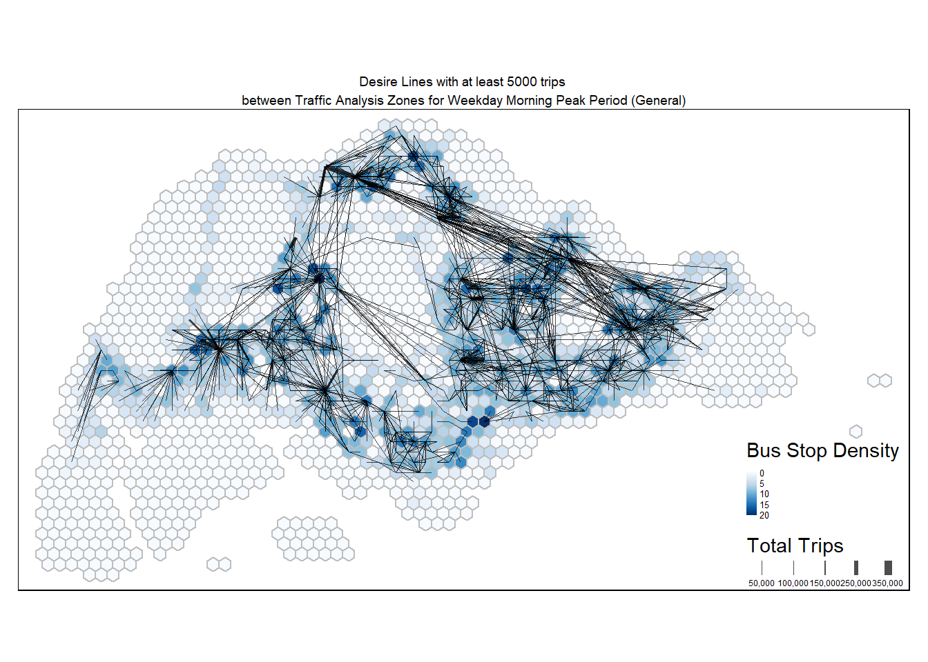
Note
Notable centroids where people are travelling to or from during weekday morning peak period include Tampines, Punggol, Jurong East, and even CBD. In terms of distances, there are several long distance routes linking the East to the North.
tm_shape(hex_grid_bounded2) +
  tm_fill(col = "busstop_count",
          palette = "Blues",
          style = "cont",
          title = "Bus Stop Density") +
  tm_borders(col = "grey") +
flowLine2 %>%
  filter(TOTAL_TRIPS >= 5000) %>%
tm_shape() +
  tm_lines(lwd = "TOTAL_TRIPS",
           style = "fixed",
           scale = c(1,2,3,4,5,7,9),
           n = 6,
           alpha = 0.7,
           title.lwd = "Total Trips") +
  tm_layout(main.title = "Desire Lines with at least 5000 trips \nbetween Traffic Analysis Zones for Weekday Morning Peak Period (November '23)",
            main.title.position = "center",
            main.title.size = 0.6,
            frame = TRUE) +
tm_legend(position = c("RIGHT", "BOTTOM"), legend.text.size = 0.4) 
tm_shape(hex_grid_bounded2) +
  tm_fill(col = "busstop_count",
          palette = "Blues",
          style = "cont",
          title = "Bus Stop Density") +
  tm_borders(col = "grey") +
flowLine3 %>%
  filter(TOTAL_TRIPS >= 5000) %>%
tm_shape() +
  tm_lines(lwd = "TOTAL_TRIPS",
           style = "fixed",
           scale = c(1,2,3,4,5,7,9),
           n = 6,
           alpha = 0.7,
           title.lwd = "Total Trips") +
  tm_layout(main.title = "Desire Lines with at least 5000 trips \nbetween Traffic Analysis Zones for Weekday Morning Peak Period (December '23)",
            main.title.position = "center",
            main.title.size = 0.6,
            frame = TRUE) +
tm_legend(position = c("RIGHT", "BOTTOM"), legend.text.size = 0.4) 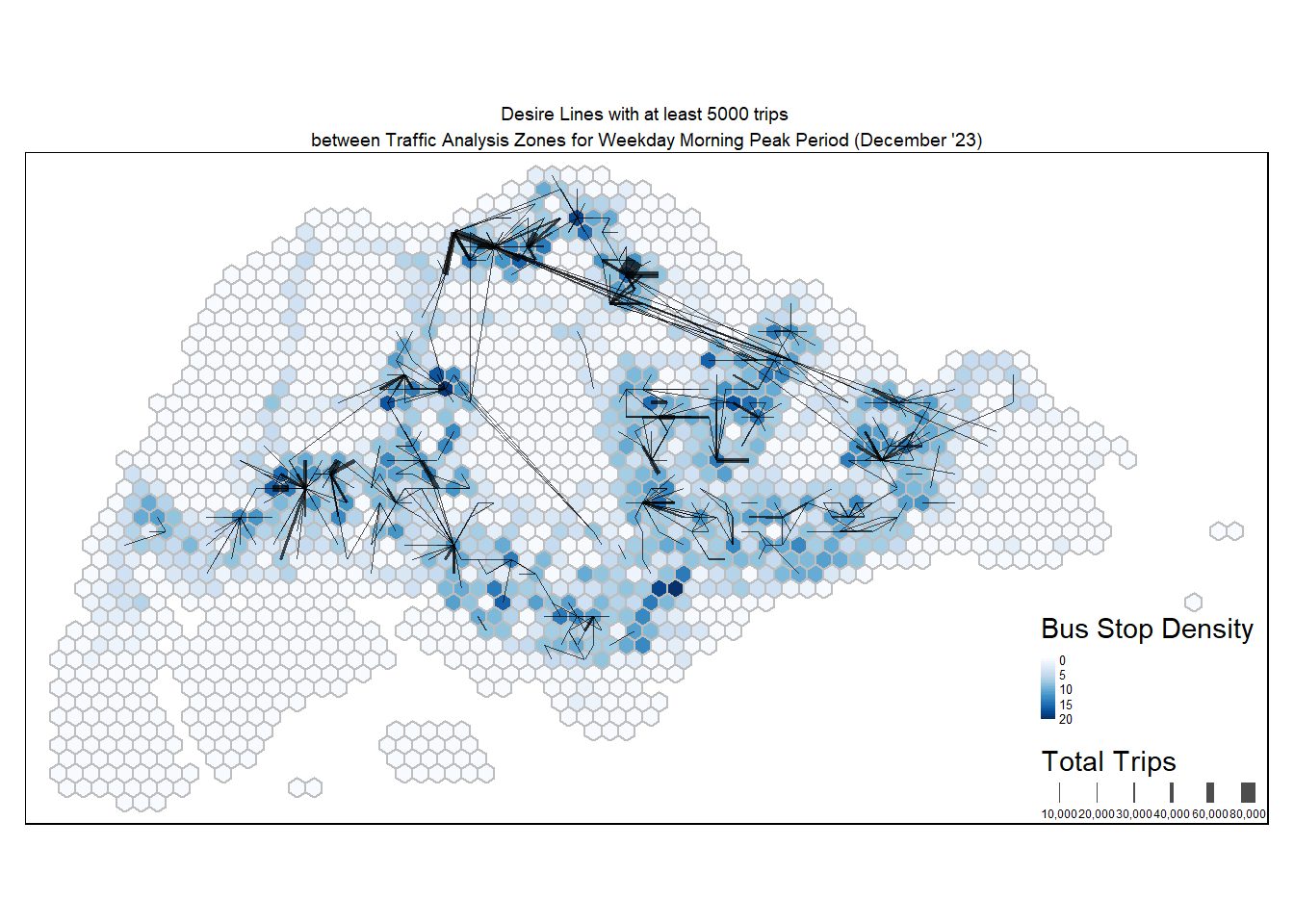
tm_shape(hex_grid_bounded2) +
  tm_fill(col = "busstop_count",
          palette = "Blues",
          style = "cont",
          title = "Bus Stop Density") +
  tm_borders(col = "grey") +
flowLine4 %>%
  filter(TOTAL_TRIPS >= 5000) %>%
tm_shape() +
  tm_lines(lwd = "TOTAL_TRIPS",
           style = "fixed",
           scale = c(1,2,3,4,5,7,9),
           n = 6,
           alpha = 0.7,
           title.lwd = "Total Trips") +
  tm_layout(main.title = "Desire Lines with at least 5000 trips \nbetween Traffic Analysis Zones for Weekday Morning Peak Period (January '24)",
            main.title.position = "center",
            main.title.size = 0.6,
            frame = TRUE) +
tm_legend(position = c("RIGHT", "BOTTOM"), legend.text.size = 0.4) 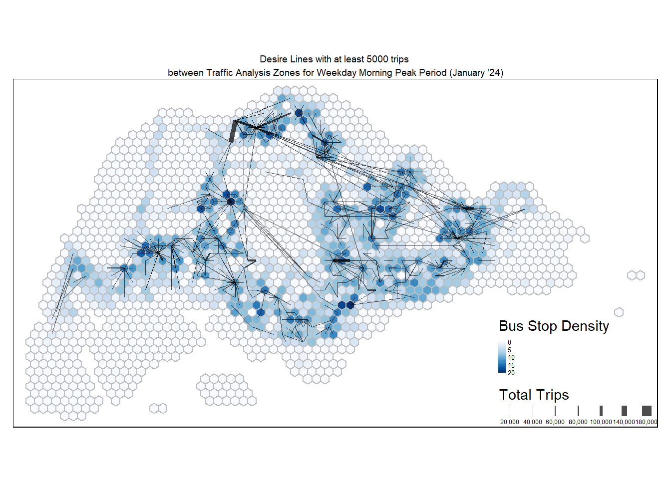
tm_shape(hex_grid_bounded2) +
  tm_fill(col = "busstop_count",
          palette = "Blues",
          style = "cont",
          title = "Bus Stop Density") +
  tm_borders(col = "grey") +
flowLine5 %>%
  filter(TOTAL_TRIPS >= 5000) %>%
tm_shape() +
  tm_lines(lwd = "TOTAL_TRIPS",
           style = "fixed",
           scale = c(1,2,3,4,5,7,9),
           n = 6,
           alpha = 0.7,
           title.lwd = "Total Trips") +
  tm_layout(main.title = "Desire Lines with at least 5000 trips \nbetween Traffic Analysis Zones for Weekday Morning Peak Period (General)",
            main.title.position = "center",
            main.title.size = 0.6,
            frame = TRUE) +
tm_legend(position = c("RIGHT", "BOTTOM"), legend.text.size = 0.4) 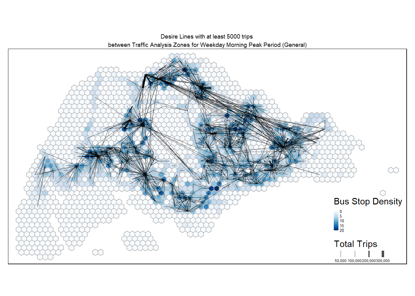
Note
Notable centroids where people are travelling to or from during weekday morning peak period include Tampines, Punggol, Jurong East, and even CBD. In terms of distances, there are several long distance routes linking the East to the North.
tm_shape(hex_grid_bounded2) +
  tm_fill(col = "busstop_count",
          palette = "Blues",
          style = "cont",
          title = "Bus Stop Density") +
  tm_borders(col = "grey") +
flowLine6 %>%
  filter(TOTAL_TRIPS >= 5000) %>%
tm_shape() +
  tm_lines(lwd = "TOTAL_TRIPS",
           style = "fixed",
           scale = c(1,2,3,4,5,7,9),
           n = 6,
           alpha = 0.7,
           title.lwd = "Total Trips") +
  tm_layout(main.title = "Desire Lines with at least 5000 trips \nbetween Traffic Analysis Zones for Weekday Morning Peak Period (November '23)",
            main.title.position = "center",
            main.title.size = 0.6,
            frame = TRUE) +
tm_legend(position = c("RIGHT", "BOTTOM"), legend.text.size = 0.4) 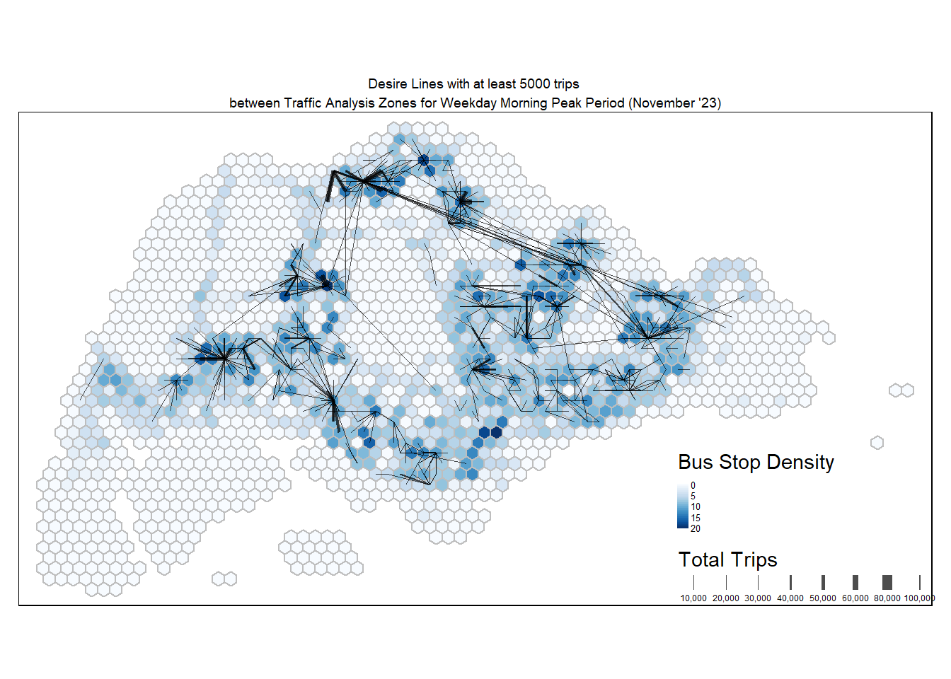
tm_shape(hex_grid_bounded2) +
  tm_fill(col = "busstop_count",
          palette = "Blues",
          style = "cont",
          title = "Bus Stop Density") +
  tm_borders(col = "grey") +
flowLine7 %>%
  filter(TOTAL_TRIPS >= 5000) %>%
tm_shape() +
  tm_lines(lwd = "TOTAL_TRIPS",
           style = "fixed",
           scale = c(1,2,3,4,5,7,9),
           n = 6,
           alpha = 0.7,
           title.lwd = "Total Trips") +
  tm_layout(main.title = "Desire Lines with at least 5000 trips \nbetween Traffic Analysis Zones for Weekday Morning Peak Period (December '23)",
            main.title.position = "center",
            main.title.size = 0.6,
            frame = TRUE) +
tm_legend(position = c("RIGHT", "BOTTOM"), legend.text.size = 0.4) 
tm_shape(hex_grid_bounded2) +
  tm_fill(col = "busstop_count",
          palette = "Blues",
          style = "cont",
          title = "Bus Stop Density") +
  tm_borders(col = "grey") +
flowLine8 %>%
  filter(TOTAL_TRIPS >= 5000) %>%
tm_shape() +
  tm_lines(lwd = "TOTAL_TRIPS",
           style = "fixed",
           scale = c(1,2,3,4,5,7,9),
           n = 6,
           alpha = 0.7,
           title.lwd = "Total Trips") +
  tm_layout(main.title = "Desire Lines with at least 5000 trips \nbetween Traffic Analysis Zones for Weekday Morning Peak Period (January '24)",
            main.title.position = "center",
            main.title.size = 0.6,
            frame = TRUE) +
tm_legend(position = c("RIGHT", "BOTTOM"), legend.text.size = 0.4) 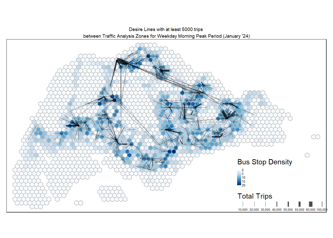
We can also zoom into individual planning areas of Singapore and observe commuting trends. A left join can be performed for hex_grid_bounded3 and mpsz using st_join() and left=TRUE. **
hex_grid_mpsz <- st_join(hex_grid_bounded2, mpsz3414, left = TRUE)

tmap_mode("view")
A filter can also then be applied on the PLN_AREA_N column to a specific planning area. Let’s look at Tampines.
hex_grid_mpsz %>%
  filter(PLN_AREA_N == "TAMPINES") %>%
tm_shape() +
  tm_fill(col = "busstop_count",
          palette = "Blues",
          style = "cont",
          title = "Bus Stop Density",
          popup.vars = c("SUBZONE_N")) +
  tm_view(set.zoom.limits = c(11,14)) +
  tm_borders(col = "grey") +
flowLine %>%
  filter(TOTAL_TRIPS >= 5000) %>%
tm_shape() +
  tm_lines(lwd = "TOTAL_TRIPS",
           style = "fixed",
           scale = c(1,2,3,4,5,7,9),
           n = 6,
           alpha = 0.7,
popup.vars = c("TOTAL_TRIPS"))tmap_mode("plot")Computing Distance Matrix
dist <- spDists(mpsz_sp,
longlat = FALSE)head(dist, n=c(10,10)) [,1] [,2] [,3] [,4] [,5] [,6]
[1,] 0.00000000 0.035282271 0.035395901 0.18199800 0.026873554 0.01286792
[2,] 0.03528227 0.000000000 0.002764531 0.14841704 0.008552614 0.04721046
[3,] 0.03539590 0.002764531 0.000000000 0.14749610 0.009403137 0.04762149
[4,] 0.18199800 0.148417042 0.147496098 0.00000000 0.156829556 0.19469772
[5,] 0.02687355 0.008552614 0.009403137 0.15682956 0.000000000 0.03866693
[6,] 0.01286792 0.047210462 0.047621487 0.19469772 0.038666929 0.00000000
[7,] 0.17287059 0.146276442 0.144315837 0.06529755 0.153255555 0.18550175
[8,] 0.13479457 0.115042375 0.112584408 0.10165987 0.120292455 0.14665912
[9,] 0.06792530 0.071740757 0.069161116 0.16564500 0.070551911 0.07590984
[10,] 0.05759682 0.044983619 0.042219355 0.13901073 0.047233657 0.06941848
[,7] [,8] [,9] [,10]
[1,] 0.17287059 0.13479457 0.06792530 0.05759682
[2,] 0.14627644 0.11504237 0.07174076 0.04498362
[3,] 0.14431584 0.11258441 0.06916112 0.04221936
[4,] 0.06529755 0.10165987 0.16564500 0.13901073
[5,] 0.15325556 0.12029246 0.07055191 0.04723366
[6,] 0.18550175 0.14665912 0.07590984 0.06941848
[7,] 0.00000000 0.05037607 0.13309198 0.11790777
[8,] 0.05037607 0.00000000 0.08514690 0.07725087
[9,] 0.13309198 0.08514690 0.00000000 0.03409883
[10,] 0.11790777 0.07725087 0.03409883 0.00000000Label column and row headers of distance matrix
Create a list sorted by planning subzone.
sz_names <- mpsz_sf$SUBZONE_NAttach the subzones to row and column for distance matrix matching.
colnames(dist) <- paste0(sz_names)
rownames(dist) <- paste0(sz_names)
Pivoting distance value by SUBZONE_N
Pivot the distance matrix into a long table by using the row and column subzone names.
distPair <- melt(dist) %>%
  rename(dist = value)
head(distPair, 10)
Var1 Var2 dist
1 MARINA EAST MARINA EAST 0.00000000
2 INSTITUTION HILL MARINA EAST 0.03528227
3 ROBERTSON QUAY MARINA EAST 0.03539590
4 JURONG ISLAND AND BUKOM MARINA EAST 0.18199800
5 FORT CANNING MARINA EAST 0.02687355
6 MARINA EAST (MP) MARINA EAST 0.01286792
7 SUDONG MARINA EAST 0.17287059
8 SEMAKAU MARINA EAST 0.13479457
9 SOUTHERN GROUP MARINA EAST 0.06792530
10 SENTOSA MARINA EAST 0.05759682- Notice that from the first row, the within zone distance is 0.
Updating intra-zonal distances
Append a constance value to replace the intra-zonaal distance of 0.
distPair %>%
  filter(dist > 0) %>%
  summary()
Var1 Var2
MARINA EAST : 331 MARINA EAST : 331
INSTITUTION HILL : 331 INSTITUTION HILL : 331
ROBERTSON QUAY : 331 ROBERTSON QUAY : 331
JURONG ISLAND AND BUKOM: 331 JURONG ISLAND AND BUKOM: 331
FORT CANNING : 331 FORT CANNING : 331
MARINA EAST (MP) : 331 MARINA EAST (MP) : 331
(Other) :107906 (Other) :107906
dist
Min. :0.001561
1st Qu.:0.064419
Median :0.107153
Mean :0.110151
3rd Qu.:0.147771
Max. :0.448634
Add a constant distance value of 50m into intra-zones distance.
distPair$dist <- ifelse(distPair$dist == 0,
                        50, distPair$dist)
Check the resulting dataframe.
distPair %>%
  summary()
Var1 Var2
MARINA EAST : 332 MARINA EAST : 332
INSTITUTION HILL : 332 INSTITUTION HILL : 332
ROBERTSON QUAY : 332 ROBERTSON QUAY : 332
JURONG ISLAND AND BUKOM: 332 JURONG ISLAND AND BUKOM: 332
FORT CANNING : 332 FORT CANNING : 332
MARINA EAST (MP) : 332 MARINA EAST (MP) : 332
(Other) :108232 (Other) :108232
dist
Min. : 0.00156
1st Qu.: 0.06455
Median : 0.10739
Mean : 0.26042
3rd Qu.: 0.14824
Max. :50.00000
Save the dataframe for future use.
write_rds(distPair, "data/rds/distPair.rds") distPair <- read_rds("data/rds/distPair.rds")Population Density
Importing Aspatial HDB data
Use read_csv() from the readr package to import the prepared HDB csv data.
hdb <- read_csv("data/aspatial/hdb.csv")

glimpse(hdb)
Rows: 12,442
Columns: 37
$ ...1 <dbl> 0, 1, 2, 3, 4, 5, 6, 7, 8, 9, 10, 11, 12, 13, 14…
$ blk_no <chr> "1", "1", "1", "1", "1", "1", "1", "1", "1", "1"…
$ street <chr> "BEACH RD", "BEDOK STH AVE 1", "CANTONMENT RD", …
$ max_floor_lvl <dbl> 16, 14, 2, 15, 4, 25, 12, 14, 12, 2, 15, 15, 13,…
$ year_completed <dbl> 1970, 1975, 2010, 1982, 1975, 1982, 1975, 1977, …
$ residential <chr> "Y", "Y", "N", "Y", "Y", "Y", "Y", "Y", "Y", "N"…
$ commercial <chr> "Y", "N", "Y", "N", "Y", "N", "N", "N", "Y", "Y"…
$ market_hawker <chr> "N", "N", "N", "N", "N", "N", "N", "N", "N", "N"…
$ miscellaneous <chr> "N", "Y", "N", "N", "N", "N", "Y", "Y", "N", "N"…
$ multistorey_carpark <chr> "N", "N", "N", "N", "N", "N", "N", "N", "N", "N"…
$ precinct_pavilion <chr> "N", "N", "N", "N", "N", "N", "N", "N", "N", "N"…
$ bldg_contract_town <chr> "KWN", "BD", "CT", "BD", "PRC", "BM", "QT", "GL"…
$ total_dwelling_units <dbl> 142, 206, 0, 102, 55, 96, 125, 247, 95, 0, 220, …
$ `1room_sold` <dbl> 0, 0, 0, 0, 0, 0, 0, 0, 0, 0, 0, 0, 0, 0, 0, 0, …
$ `2room_sold` <dbl> 1, 0, 0, 0, 0, 0, 0, 0, 0, 0, 0, 0, 0, 0, 0, 0, …
$ `3room_sold` <dbl> 138, 204, 0, 0, 54, 0, 118, 0, 62, 0, 216, 214, …
$ `4room_sold` <dbl> 1, 0, 0, 10, 0, 0, 0, 0, 0, 0, 0, 0, 0, 0, 0, 0,…
$ `5room_sold` <dbl> 2, 2, 0, 92, 1, 96, 7, 0, 33, 0, 4, 5, 0, 4, 0, …
$ exec_sold <dbl> 0, 0, 0, 0, 0, 0, 0, 0, 0, 0, 0, 0, 0, 0, 0, 0, …
$ multigen_sold <dbl> 0, 0, 0, 0, 0, 0, 0, 0, 0, 0, 0, 0, 0, 0, 0, 0, …
$ studio_apartment_sold <dbl> 0, 0, 0, 0, 0, 0, 0, 0, 0, 0, 0, 0, 0, 0, 0, 0, …
$ `1room_rental` <dbl> 0, 0, 0, 0, 0, 0, 0, 0, 0, 0, 0, 0, 319, 0, 0, 0…
$ `2room_rental` <dbl> 0, 0, 0, 0, 0, 0, 0, 247, 0, 0, 0, 0, 0, 0, 56, …
$ `3room_rental` <dbl> 0, 0, 0, 0, 0, 0, 0, 0, 0, 0, 0, 0, 0, 0, 14, 1,…
$ other_room_rental <dbl> 0, 0, 0, 0, 0, 0, 0, 0, 0, 0, 0, 0, 0, 0, 14, 0,…
$ lat <dbl> 1.295097, 1.320852, 1.275488, 1.327969, 1.388610…
$ lng <dbl> 103.8541, 103.9337, 103.8414, 103.9227, 103.9881…
$ building <chr> "RAFFLES HOTEL", "NIL", "PINNACLE @ DUXTON", "PI…
$ addr <chr> "1 BEACH ROAD RAFFLES HOTEL SINGAPORE 189673", "…
$ postal <chr> "189673", "460001", "080001", "461001", "500001"…
$ SUBZONE_NO <dbl> 2, 6, 3, 3, 1, 9, 10, 5, 3, 5, 1, 5, 2, 2, 1, 7,…
$ SUBZONE_N <chr> "CITY HALL", "BEDOK SOUTH", "CHINATOWN", "KEMBAN…
$ SUBZONE_C <chr> "DTSZ02", "BDSZ06", "OTSZ03", "BDSZ03", "CHSZ01"…
$ PLN_AREA_N <chr> "DOWNTOWN CORE", "BEDOK", "OUTRAM", "BEDOK", "CH…
$ PLN_AREA_C <chr> "DT", "BD", "OT", "BD", "CH", "BM", "QT", "GL", …
$ REGION_N <chr> "CENTRAL REGION", "EAST REGION", "CENTRAL REGION…
$ REGION_C <chr> "CR", "ER", "CR", "ER", "ER", "CR", "CR", "CR", …For the purpose of computing a proxy for population density, the residential units will be extracted using filter() from the dplyr package.
hdb_residential <- hdb %>%
  filter(residential == "Y")

head(hdb_residential, 10)
# A tibble: 10 × 37
...1 blk_no street max_floor_lvl year_completed residential commercial
<dbl> <chr> <chr> <dbl> <dbl> <chr> <chr>
1 0 1 BEACH RD 16 1970 Y Y
2 1 1 BEDOK STH A… 14 1975 Y N
3 3 1 CHAI CHEE RD 15 1982 Y N
4 4 1 CHANGI VILL… 4 1975 Y Y
5 5 1 DELTA AVE 25 1982 Y N
6 6 1 DOVER RD 12 1975 Y N
7 7 1 EUNOS CRES 14 1977 Y N
8 8 1 EVERTON PK 12 1980 Y Y
9 10 1 GHIM MOH RD 15 1975 Y N
10 11 1 HAIG RD 15 1976 Y N
# ℹ 30 more variables: market_hawker <chr>, miscellaneous <chr>,
# multistorey_carpark <chr>, precinct_pavilion <chr>,
# bldg_contract_town <chr>, total_dwelling_units <dbl>, `1room_sold` <dbl>,
# `2room_sold` <dbl>, `3room_sold` <dbl>, `4room_sold` <dbl>,
# `5room_sold` <dbl>, exec_sold <dbl>, multigen_sold <dbl>,
# studio_apartment_sold <dbl>, `1room_rental` <dbl>, `2room_rental` <dbl>,
# `3room_rental` <dbl>, other_room_rental <dbl>, lat <dbl>, lng <dbl>, …There are also some outliers like hotels that are classified as a residential unit. We can remove rows containing ‘hotel’ using grepl().
hotels <- hdb_residential %>%
  filter(grepl("HOTEL", building, ignore.case = TRUE))

kable(hotels)| …1 | blk_no | street | max_floor_lvl | year_completed | residential | commercial | market_hawker | miscellaneous | multistorey_carpark | precinct_pavilion | bldg_contract_town | total_dwelling_units | 1room_sold | 2room_sold | 3room_sold | 4room_sold | 5room_sold | exec_sold | multigen_sold | studio_apartment_sold | 1room_rental | 2room_rental | 3room_rental | other_room_rental | lat | lng | building | addr | postal | SUBZONE_NO | SUBZONE_N | SUBZONE_C | PLN_AREA_N | PLN_AREA_C | REGION_N | REGION_C |
|---|---|---|---|---|---|---|---|---|---|---|---|---|---|---|---|---|---|---|---|---|---|---|---|---|---|---|---|---|---|---|---|---|---|---|---|---|
| 0 | 1 | BEACH RD | 16 | 1970 | Y | Y | N | N | N | N | KWN | 142 | 0 | 1 | 138 | 1 | 2 | 0 | 0 | 0 | 0 | 0 | 0 | 0 | 1.295097 | 103.8541 | RAFFLES HOTEL | 1 BEACH ROAD RAFFLES HOTEL SINGAPORE 189673 | 189673 | 2 | CITY HALL | DTSZ02 | DOWNTOWN CORE | DT | CENTRAL REGION | CR |
| 4580 | 3 | BEACH RD | 16 | 1970 | Y | Y | N | N | N | N | KWN | 138 | 0 | 1 | 134 | 0 | 3 | 0 | 0 | 0 | 0 | 0 | 0 | 0 | 1.294801 | 103.8545 | RAFFLES HOTEL SINGAPORE | 3 BEACH ROAD RAFFLES HOTEL SINGAPORE SINGAPORE 189674 | 189674 | 2 | CITY HALL | DTSZ02 | DOWNTOWN CORE | DT | CENTRAL REGION | CR |
The HDB Blk 1 Beach Road shares a similar address as Raffles Hotel’s 1 Beach Road, but they have different postal codes.
To verify other similar addresses, filter for addresses containing “BEACH RD”.
beach_rd <- hdb_residential %>%
  filter(grepl("BEACH RD", street, ignore.case = TRUE))

kable(beach_rd)| …1 | blk_no | street | max_floor_lvl | year_completed | residential | commercial | market_hawker | miscellaneous | multistorey_carpark | precinct_pavilion | bldg_contract_town | total_dwelling_units | 1room_sold | 2room_sold | 3room_sold | 4room_sold | 5room_sold | exec_sold | multigen_sold | studio_apartment_sold | 1room_rental | 2room_rental | 3room_rental | other_room_rental | lat | lng | building | addr | postal | SUBZONE_NO | SUBZONE_N | SUBZONE_C | PLN_AREA_N | PLN_AREA_C | REGION_N | REGION_C |
|---|---|---|---|---|---|---|---|---|---|---|---|---|---|---|---|---|---|---|---|---|---|---|---|---|---|---|---|---|---|---|---|---|---|---|---|---|
| 0 | 1 | BEACH RD | 16 | 1970 | Y | Y | N | N | N | N | KWN | 142 | 0 | 1 | 138 | 1 | 2 | 0 | 0 | 0 | 0 | 0 | 0 | 0 | 1.295097 | 103.8541 | RAFFLES HOTEL | 1 BEACH ROAD RAFFLES HOTEL SINGAPORE 189673 | 189673 | 2 | CITY HALL | DTSZ02 | DOWNTOWN CORE | DT | CENTRAL REGION | CR |
| 1660 | 15 | BEACH RD | 20 | 1974 | Y | Y | N | N | N | N | KWN | 76 | 0 | 0 | 0 | 76 | 0 | 0 | 0 | 0 | 0 | 0 | 0 | 0 | 1.295796 | 103.8555 | NIL | 15 BEACH ROAD | NIL | 1 | BUGIS | DTSZ01 | DOWNTOWN CORE | DT | CENTRAL REGION | CR |
| 2079 | 17 | BEACH RD | 20 | 1974 | Y | Y | N | N | N | N | KWN | 76 | 0 | 0 | 0 | 76 | 0 | 0 | 0 | 0 | 0 | 0 | 0 | 0 | 1.303689 | 103.8636 | GOLDEN BEACH VISTA | 17 BEACH ROAD GOLDEN BEACH VISTA SINGAPORE 190017 | 190017 | 9 | CRAWFORD | KLSZ09 | KALLANG | KL | CENTRAL REGION | CR |
| 2567 | 2 | BEACH RD | 16 | 1970 | Y | Y | N | N | N | N | KWN | 139 | 0 | 1 | 136 | 0 | 2 | 0 | 0 | 0 | 0 | 0 | 0 | 0 | 1.390462 | 103.9753 | CHANGI BEACH CLUB | 2 ANDOVER ROAD CHANGI BEACH CLUB SINGAPORE 509984 | 509984 | 1 | CHANGI POINT | CHSZ01 | CHANGI | CH | EAST REGION | ER |
| 4580 | 3 | BEACH RD | 16 | 1970 | Y | Y | N | N | N | N | KWN | 138 | 0 | 1 | 134 | 0 | 3 | 0 | 0 | 0 | 0 | 0 | 0 | 0 | 1.294801 | 103.8545 | RAFFLES HOTEL SINGAPORE | 3 BEACH ROAD RAFFLES HOTEL SINGAPORE SINGAPORE 189674 | 189674 | 2 | CITY HALL | DTSZ02 | DOWNTOWN CORE | DT | CENTRAL REGION | CR |
| 6028 | 4 | BEACH RD | 16 | 1968 | Y | N | N | Y | N | N | KWN | 336 | 0 | 0 | 0 | 0 | 0 | 0 | 0 | 0 | 336 | 0 | 0 | 0 | 1.304716 | 103.8652 | NIL | 4 BEACH ROAD SINGAPORE 190004 | 190004 | 9 | CRAWFORD | KLSZ09 | KALLANG | KL | CENTRAL REGION | CR |
| 7743 | 5 | BEACH RD | 16 | 1968 | Y | N | N | Y | N | N | KWN | 336 | 0 | 0 | 0 | 0 | 0 | 0 | 0 | 0 | 336 | 0 | 0 | 0 | 1.298092 | 103.8569 | BEACH ROAD CONSERVATION AREA | 5 TAN QUEE LAN STREET BEACH ROAD CONSERVATION AREA SINGAPORE 188094 | 188094 | 1 | BUGIS | DTSZ01 | DOWNTOWN CORE | DT | CENTRAL REGION | CR |
| 8956 | 6 | BEACH RD | 16 | 1968 | Y | Y | N | N | N | N | KWN | 198 | 0 | 45 | 1 | 28 | 0 | 0 | 0 | 0 | 57 | 67 | 0 | 0 | 1.303992 | 103.8644 | BEACH ROAD GARDENS | 6 BEACH ROAD BEACH ROAD GARDENS SINGAPORE 190006 | 190006 | 9 | CRAWFORD | KLSZ09 | KALLANG | KL | CENTRAL REGION | CR |
2, 5 and 15 Beach Road do not have the correct postal codes following the 1900XX convention. Additionally, these addresses do not have the correct coordinates too.
With reference to URA’s official asset map of Singapore, OneMap, the data will be manually modified using mutate() and ifelse().
hdb_residential2 <- hdb_residential %>%
  mutate(postal = ifelse(blk_no == 1 & street == "BEACH RD", 190001, postal)) %>%
  mutate(lat = ifelse(blk_no == 1 & street == "BEACH RD", 1.3036714, lat)) %>%
  mutate(lng = ifelse(blk_no == 1 & street == "BEACH RD", 103.8644787, lng)) %>%
  mutate(postal = ifelse(blk_no == 2 & street == "BEACH RD", 190002, postal)) %>%
  mutate(lat = ifelse(blk_no == 2 & street == "BEACH RD", 1.3040331, lat)) %>%
  mutate(lng = ifelse(blk_no == 2 & street == "BEACH RD", 103.8649285, lng)) %>%
  mutate(postal = ifelse(blk_no == 3 & street == "BEACH RD", 190003, postal)) %>%
  mutate(lat = ifelse(blk_no == 3 & street == "BEACH RD", 1.3041872, lat)) %>%
  mutate(lng = ifelse(blk_no == 3 & street == "BEACH RD", 103.8651934, lng)) %>%
  mutate(postal = ifelse(blk_no == 5 & street == "BEACH RD", 190005, postal)) %>%
  mutate(lat = ifelse(blk_no == 5 & street == "BEACH RD", 1.3043463, lat)) %>%
  mutate(lng = ifelse(blk_no == 5 & street == "BEACH RD", 103.8648158, lng)) %>%
  mutate(postal = ifelse(blk_no == 15 & street == "BEACH RD", 190015, postal)) %>%
  mutate(lat = ifelse(blk_no == 15 & street == "BEACH RD", 1.3034254, lat)) %>%
  mutate(lng = ifelse(blk_no == 15 & street == "BEACH RD", 103.8631535, lng))
Check for any duplicates.
duplicate <- hdb_residential2 %>%
  group_by_all() %>%
  filter(n()>1) %>%
  ungroup()

DT::datatable(duplicate)
Converting Aspatial data to Geospatial data
Longitude and latitude values are in decimal degrees and thus the data is in wgs84 geographic coordinate system.
To convert hdb_residential2 into sf, we use st_as_sf() and set the crs argument to 4326 first. The transformation to Singapore’s coordinate reference system 3414 will be done with st_transform().
We only need the postal code, total dwelling units and geometry attributes so we will use the select() function to extract these columns.
hdb_residential_sf <- st_as_sf(hdb_residential2,
                   coords = c("lng", "lat"),
                   crs=4326) %>%
  st_transform(crs = 3414) %>%
  select(postal, total_dwelling_units, geometry)

str(hdb_residential_sf)
sf [10,181 × 3] (S3: sf/tbl_df/tbl/data.frame)
$ postal : chr [1:10181] "190001" "460001" "461001" "500001" ...
$ total_dwelling_units: num [1:10181] 142 206 102 55 96 125 247 95 220 219 ...
$ geometry :sfc_POINT of length 10181; first list element: 'XY' num [1:2] 31468 31779
- attr(*, "sf_column")= chr "geometry"
- attr(*, "agr")= Factor w/ 3 levels "constant","aggregate",..: NA NA
..- attr(*, "names")= chr [1:2] "postal" "total_dwelling_units"Let’s build the HDB residential population density map.
tm_shape(hex_grid_bounded2) +
  tm_fill(col = "busstop_count",
          palette = "Blues",
          style = "cont",
          title = "Bus Stop Density") +
  tm_borders(col = "grey") +
tm_shape(hdb_residential_sf) +
  tm_dots() +
  tm_layout(main.title = "Location of HDB Residential Units",
            main.title.position = "center",
            main.title.size = 1,
            frame = TRUE)  +
  tm_legend(position = c("RIGHT", "BOTTOM"), legend.text.size = 0.4)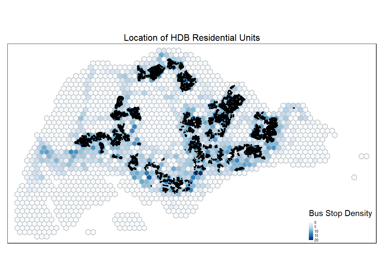
Performming in-polygon count
housing_count <- st_join(hex_grid_bounded2, hdb_residential_sf,
                     join = st_intersects, left = TRUE) %>%
  st_drop_geometry() %>%
  group_by(index) %>%
  summarise(housing_count = sum(total_dwelling_units)) %>%
  ungroup() %>%
  mutate(housing_count = ifelse(is.na(housing_count), 0, housing_count))
hex_grid_bounded3 <- left_join(hex_grid_bounded2, housing_count,
by = c("index" = "index"))
summary(hex_grid_bounded3$housing_count) Min. 1st Qu. Median Mean 3rd Qu. Max.
0 0 0 652 0 7879 tm_shape(hex_grid_bounded3) +
tm_fill(col = "housing_count",
palette = "Blues",
style = "cont",
title = "Housing Density") +
tm_borders(col = "grey") +
tm_legend(position = c("RIGHT", "BOTTOM"), legend.text.size = 0.4)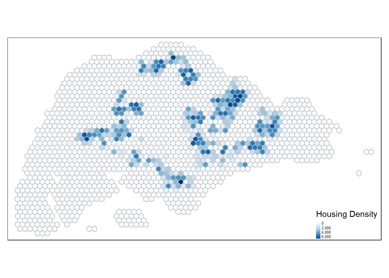
Employment Opportunities Density
Import Geospatial data: Business
biz <- st_read("data/geospatial/Business.shp") %>% st_transform(crs=3414)Reading layer `Business' from data source
`C:\guacodemoleh\IS415-GAA\Take-home_Ex\Take-home_Ex03\data\geospatial\Business.shp'
using driver `ESRI Shapefile'
Simple feature collection with 6550 features and 3 fields
Geometry type: POINT
Dimension: XY
Bounding box: xmin: 3669.148 ymin: 25408.41 xmax: 47034.83 ymax: 50148.54
Projected CRS: SVY21 / Singapore TMtm_shape(hex_grid_bounded3) +
tm_fill(col = "busstop_count",
palette = "Blues",
style = "cont",
title = "Bus Stop Density") +
tm_borders(col = "grey") +
tm_shape(biz) +
tm_dots() +
tm_layout(main.title = "Location of Businesses",
main.title.position = "center",
main.title.size = 1,
frame = TRUE) +
tm_legend(position = c("RIGHT", "BOTTOM"), legend.text.size = 0.4)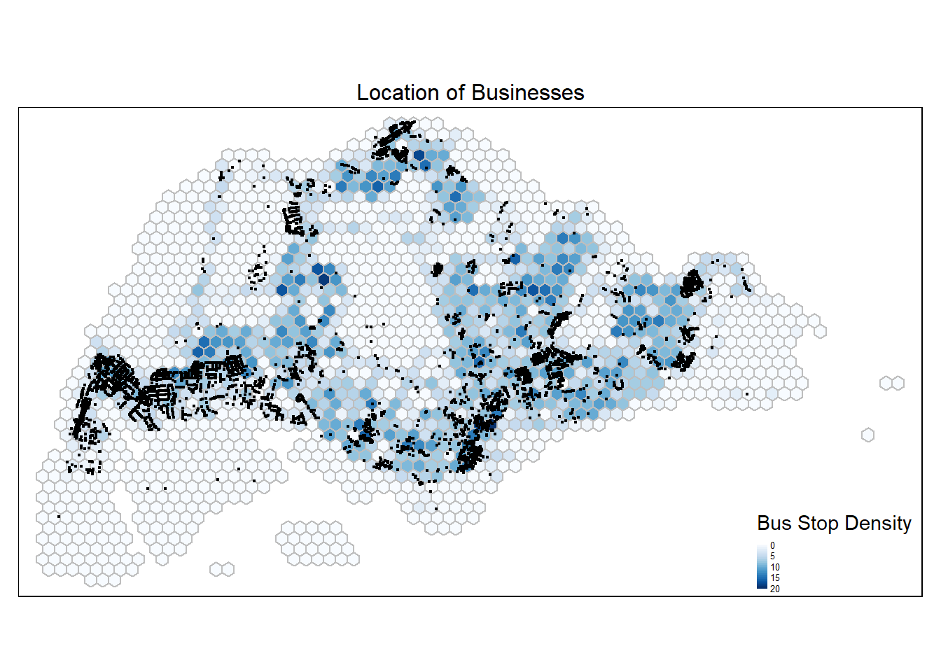
Businesses are concentrated in the central and west regions.
Perform point-in-polygon count
hex_grid_bounded3$biz_count <- lengths(st_intersects(hex_grid_bounded3, biz))

summary(hex_grid_bounded3$biz_count)
Min. 1st Qu. Median Mean 3rd Qu. Max.
0.000 0.000 0.000 3.915 2.000 106.000 tm_shape(hex_grid_bounded3) +
tm_fill(col = "biz_count",
palette = "Blues",
style = "cont",
title = "Business Density") +
tm_borders(col = "grey") +
tm_legend(position = c("RIGHT", "BOTTOM"), legend.text.size = 0.4)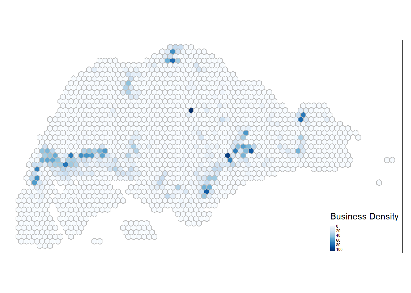
Schools Density
schools <- read_csv("data/aspatial/schoolsclean.csv")schools <- schools %>%
separate(latlong, into = c("latitude", "longitude"), sep = ",", convert = TRUE)
schools_sf <- st_as_sf(schools, coords = c("longitude","latitude"), crs = 4326) %>%
st_transform(crs=3414)tm_shape(hex_grid_bounded3) +
tm_fill(col = "busstop_count",
palette = "Blues",
style = "cont",
title = "Bus Stop Density") +
tm_borders(col = "grey") +
tm_shape(schools_sf) +
tm_dots() +
tm_layout(main.title = "Location of Schools",
main.title.position = "center",
main.title.size = 1,
frame = TRUE) +
tm_legend(position = c("RIGHT", "BOTTOM"), legend.text.size = 0.4)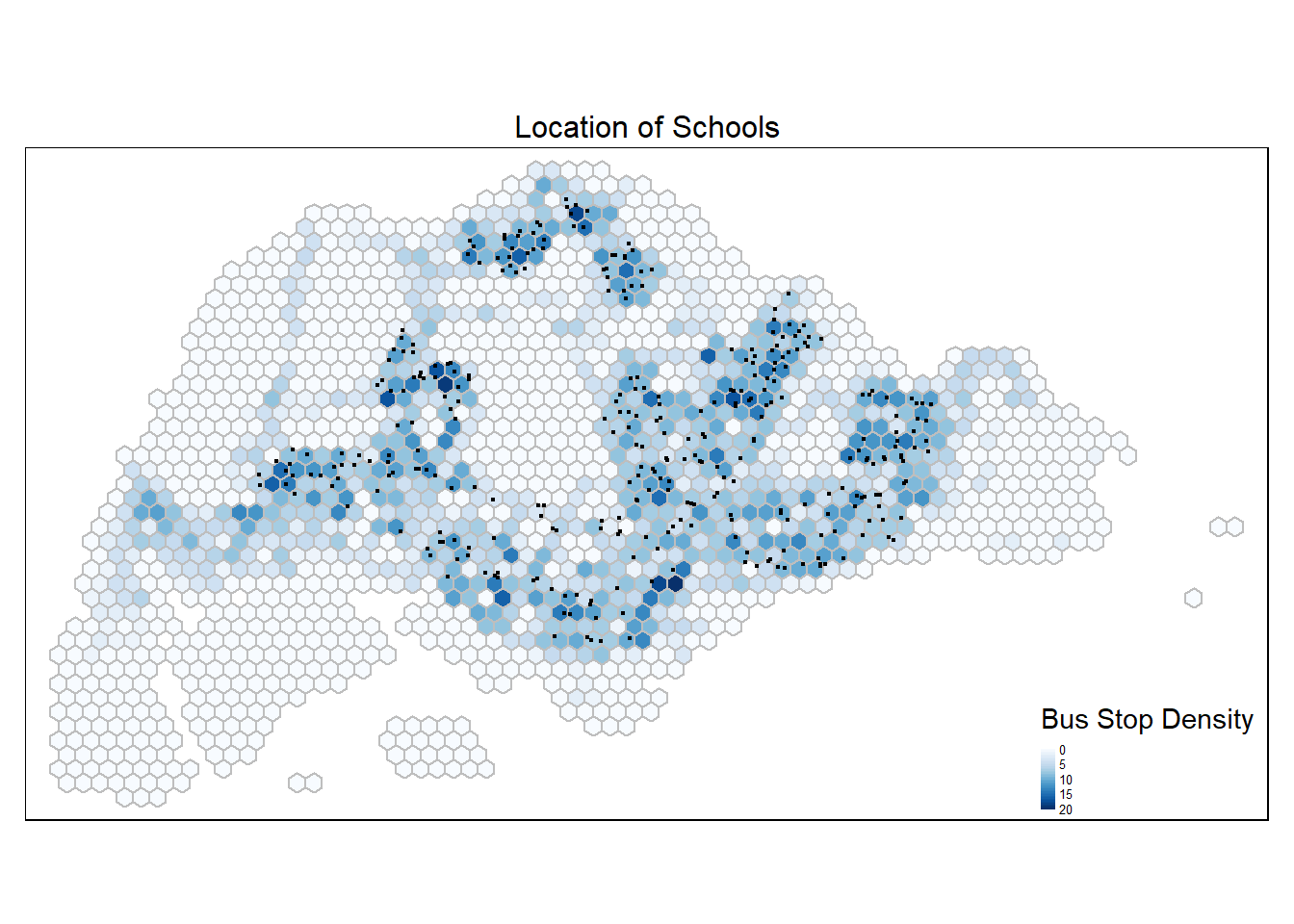
Perform point-in-polygon count
hex_grid_bounded3$school_count <- lengths(st_intersects(hex_grid_bounded3, schools_sf))

summary(hex_grid_bounded3$school_count)
Min. 1st Qu. Median Mean 3rd Qu. Max.
0.0000 0.0000 0.0000 0.1943 0.0000 4.0000 tm_shape(hex_grid_bounded3) +
tm_fill(col = "school_count",
palette = "Blues",
style = "cont",
title = "School Density") +
tm_borders(col = "grey") +
tm_legend(position = c("RIGHT", "BOTTOM"), legend.text.size = 0.4)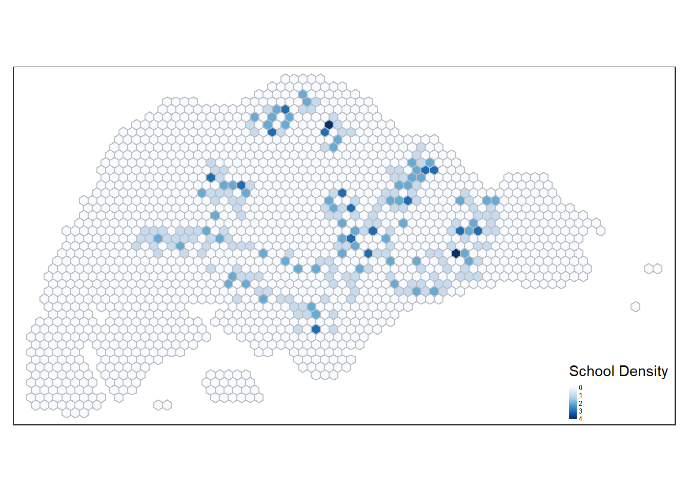
Financial Services Density
Importing Geospatial data: Fenancial Services
FinServ <- st_read(dsn = "data/geospatial", layer = "FinServ") %>%
  st_transform(crs = 3414)
Reading layer `FinServ' from data source
`C:\guacodemoleh\IS415-GAA\Take-home_Ex\Take-home_Ex03\data\geospatial'
using driver `ESRI Shapefile'
Simple feature collection with 3320 features and 3 fields
Geometry type: POINT
Dimension: XY
Bounding box: xmin: 4881.527 ymin: 25171.88 xmax: 46526.16 ymax: 49338.02
Projected CRS: SVY21 / Singapore TMtm_shape(hex_grid_bounded3) +
tm_fill(col = "busstop_count",
palette = "Blues",
style = "cont",
title = "Bus Stop Density") +
tm_borders(col = "grey") +
tm_shape(FinServ) +
tm_dots() +
tm_layout(main.title = "Location of Financial Services",
main.title.position = "center",
main.title.size = 1,
frame = TRUE) +
tm_legend(position = c("RIGHT", "BOTTOM"), legend.text.size = 0.4)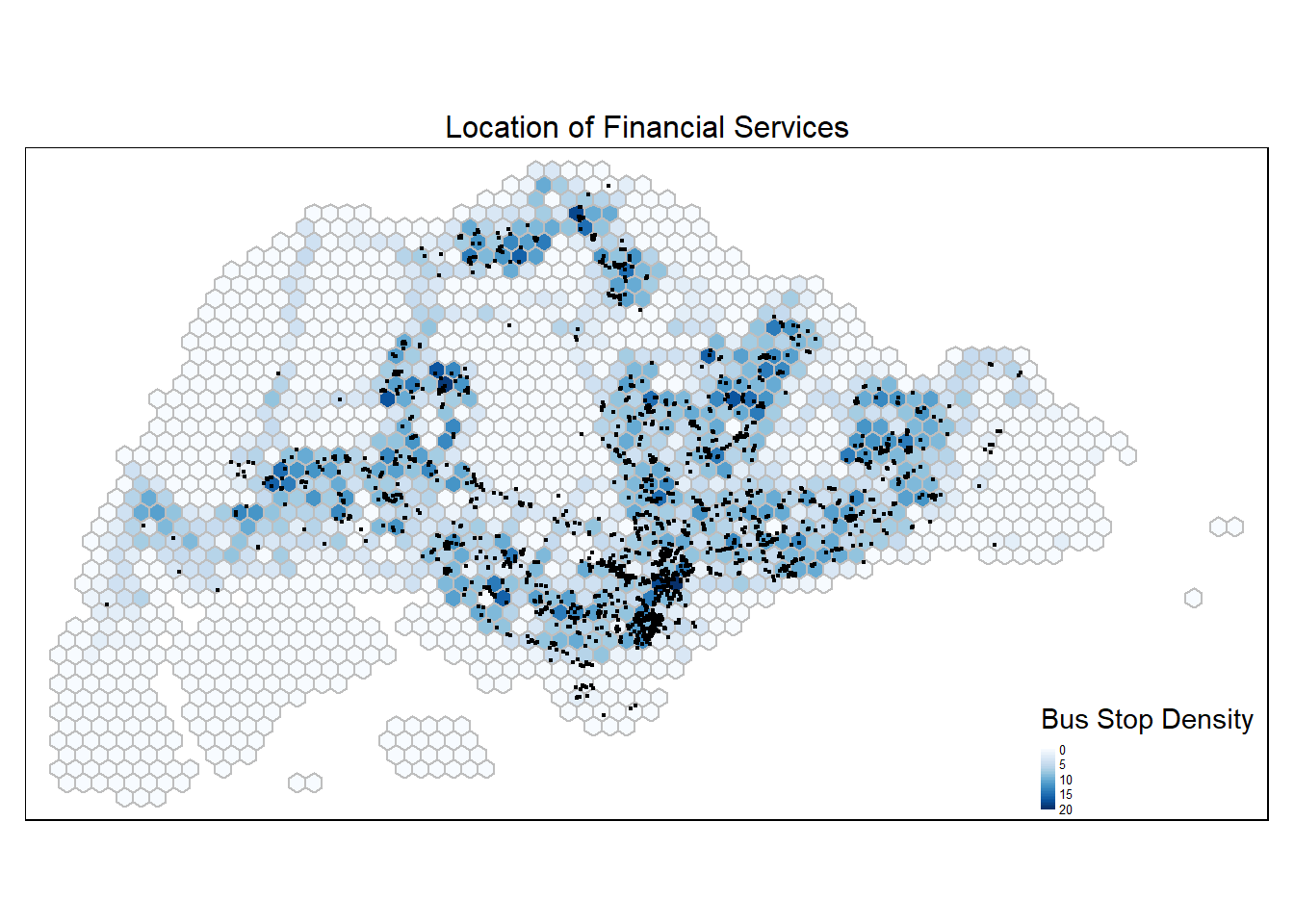
Perform point-in-polygon count
hex_grid_bounded3$fin_count <- lengths(st_intersects(hex_grid_bounded3, FinServ))

summary(hex_grid_bounded3$fin_count)
Min. 1st Qu. Median Mean 3rd Qu. Max.
0.000 0.000 0.000 1.984 1.000 117.000 tm_shape(hex_grid_bounded3) +
tm_fill(col = "fin_count",
palette = "Blues",
style = "cont",
title = "Financial Services Density") +
tm_borders(col = "grey") +
tm_legend(position = c("RIGHT", "BOTTOM"), legend.text.size = 0.4)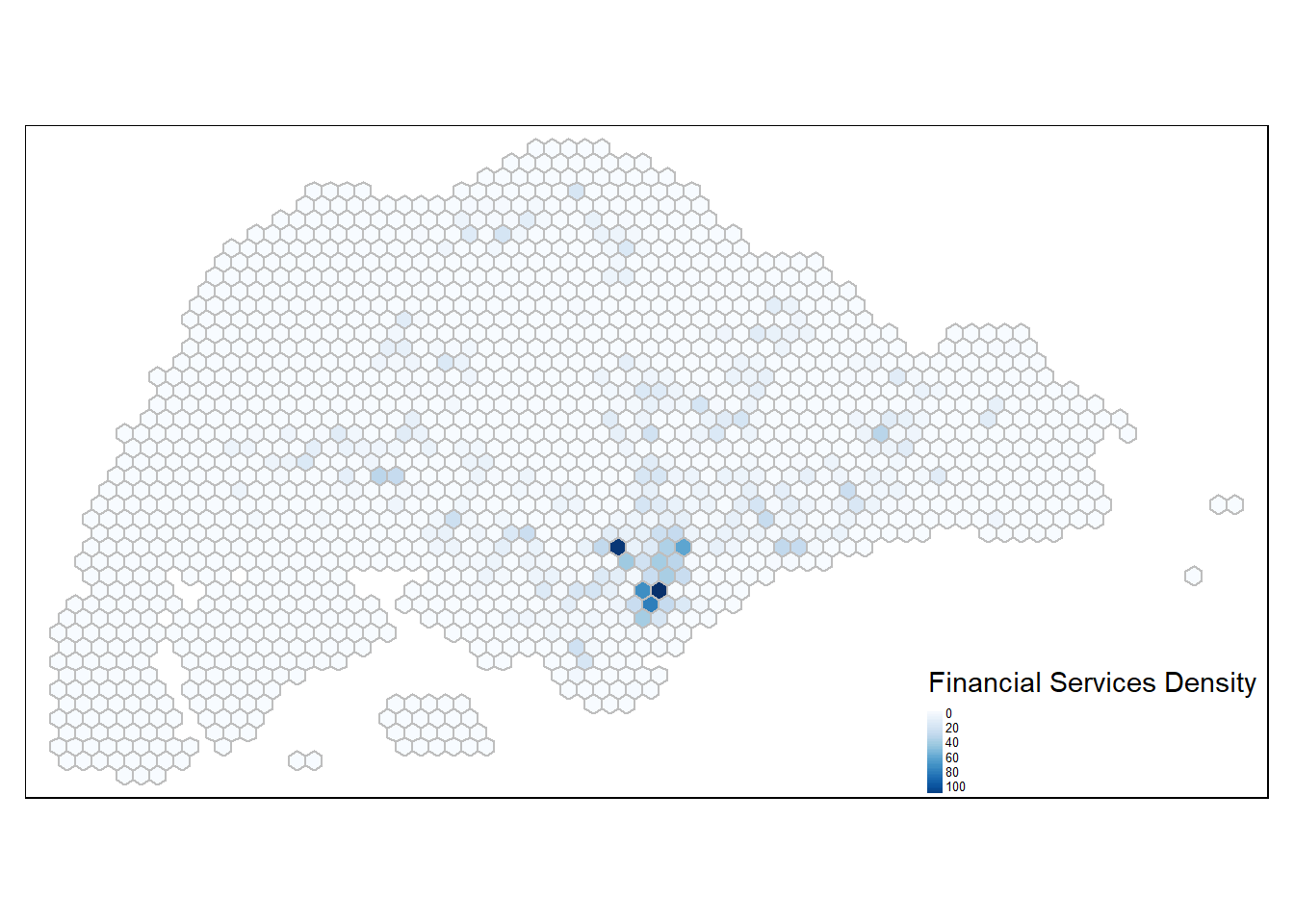
Public Healthcare Density
public_hc <- read_csv("data/aspatial/HospitalsPolyclinics v_2024.csv")public_hc.sf <- st_as_sf(public_hc[1:42,], wkt = "geometry", crs = 4326) %>%
st_transform(crs=3414)
public_hc2.sf <- st_as_sf(public_hc[43:1235,], wkt = "geometry", crs = 3414) # CHAS clinics encoded in EPSG 3414
public_hc.sf <- rbind(public_hc.sf, public_hc2.sf)
write_rds(public_hc.sf, "data/geospatial/public_hc.sf")Perform point-in-polygon count
hex_grid_bounded3$hc_count <- lengths(st_intersects(hex_grid_bounded3, public_hc.sf))

summary(hex_grid_bounded3$fin_count)
Min. 1st Qu. Median Mean 3rd Qu. Max.
0.000 0.000 0.000 1.984 1.000 117.000 tm_shape(hex_grid_bounded3) +
tm_fill(col = "hc_count",
palette = "Blues",
style = "cont",
title = "Public Healthcare Services Density") +
tm_borders(col = "grey") +
tm_legend(position = c("RIGHT", "BOTTOM"), legend.text.size = 0.4)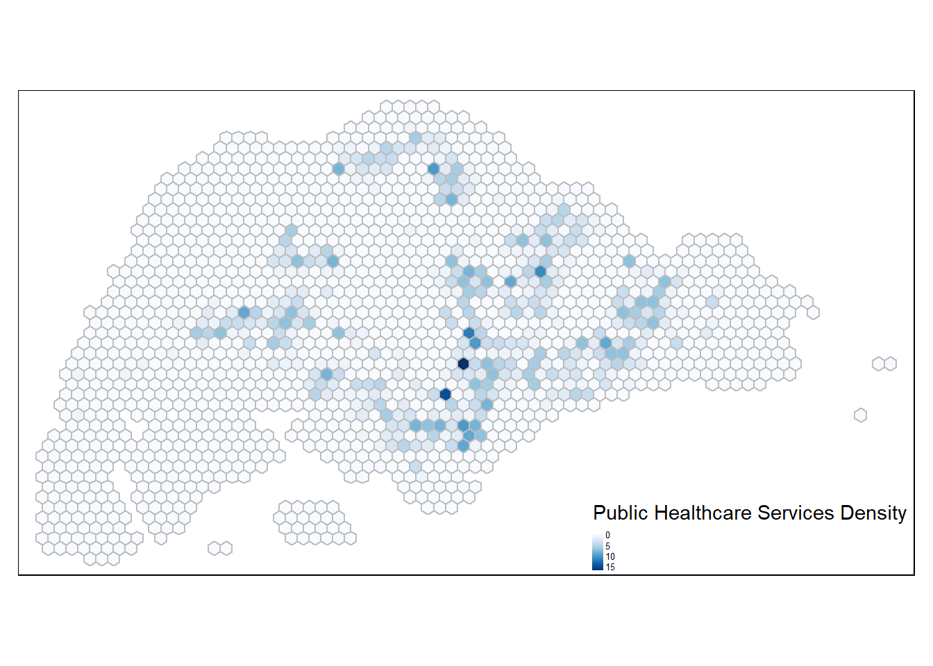
Prepare origin variables
propulsive <- hex_grid_bounded3 %>%
  st_drop_geometry() %>%
  select(index, biz_count, school_count, fin_count, hc_count, busstop_count)


origin <- names(propulsive) %>%
  modify_at(-1, ~ paste0("o_", .))  # Add prefix to all except index

# Assign modified names back to the data frame
names(propulsive) <- origin
Prepare destination variables
The attractiveness variables will be compiled into a tibble data frame called attractiveness to be used for the Spatial Interaction Model later. A prefix of “d_” will be added to the column names to identify them as origin variables.
attractiveness <- hex_grid_bounded3 %>%
  st_drop_geometry() %>%
  select(index, biz_count, school_count, fin_count, hc_count, busstop_count)

destin <- names(attractiveness) %>%
  modify_at(-1, ~ paste0("d_", .)) # index no prefix added
Compute Distance Matrix
In spatial interaction, a distance matrix is a table that shows the distance between pairs of locations. A location’s distance from itself, which is shown in the main diagonal of a distance matrix table, is 0.
There are at least two ways to compute the required distance matrix – one based on sf and the other based on sp. However, past experience has shown that computing the distance matrix using sf function takes relatively longer than sp method especially when the data set is large. In view of this, sp method will be used in the code chunks below.
Converting sf data frame to SpatialPolygonsDataFrame
hex_grid_sp <- as(hex_grid_bounded2, "Spatial")
hex_grid_sp
class : SpatialPolygonsDataFrame
features : 1673
extent : 2292.538, 56667.54, 21015.46, 50460.32 (xmin, xmax, ymin, ymax)
crs : +proj=tmerc +lat_0=1.36666666666667 +lon_0=103.833333333333 +k=1 +x_0=28001.642 +y_0=38744.572 +ellps=WGS84 +towgs84=0,0,0,0,0,0,0 +units=m +no_defs
variables : 2
names : index, busstop_count
min values : 100, 0
max values : 999, 20 The code chunk below is used to measure the distance between the central points of each pair of spatial shapes using the function spDists() of sp package. This method is widely used due to its computational simplicity, providing a reasonably accurate indication of spatial connections between the shapes. As mentioned above, calculating distances between centroids demands less computational resources than calculations between all points along polygon edges, especially for intricate polygons with many vertices. Centroids also act as single point representations that provide an overview of the shape. While edges offer intricate shape details, the generalized perspective of centroids could be valuable when precise edge shapes are less critical.
dist <- spDists(hex_grid_sp, longlat = FALSE)

# Examine the resultant matrix
head(dist, n=c(10, 10))
[,1] [,2] [,3] [,4] [,5] [,6] [,7] [,8]
[1,] 0.000 1299.038 2598.076 3897.114 5196.152 750.000 750.000 1984.313
[2,] 1299.038 0.000 1299.038 2598.076 3897.114 1984.313 750.000 750.000
[3,] 2598.076 1299.038 0.000 1299.038 2598.076 3269.174 1984.313 750.000
[4,] 3897.114 2598.076 1299.038 0.000 1299.038 4562.072 3269.174 1984.313
[5,] 5196.152 3897.114 2598.076 1299.038 0.000 5857.687 4562.072 3269.174
[6,] 750.000 1984.313 3269.174 4562.072 5857.687 0.000 1299.038 2598.076
[7,] 750.000 750.000 1984.313 3269.174 4562.072 1299.038 0.000 1299.038
[8,] 1984.313 750.000 750.000 1984.313 3269.174 2598.076 1299.038 0.000
[9,] 3269.174 1984.313 750.000 750.000 1984.313 3897.114 2598.076 1299.038
[10,] 4562.072 3269.174 1984.313 750.000 750.000 5196.152 3897.114 2598.076
[,9] [,10]
[1,] 3269.174 4562.072
[2,] 1984.313 3269.174
[3,] 750.000 1984.313
[4,] 750.000 750.000
[5,] 1984.313 750.000
[6,] 3897.114 5196.152
[7,] 2598.076 3897.114
[8,] 1299.038 2598.076
[9,] 0.000 1299.038
[10,] 1299.038 0.000As seen in the output above, the result is a matrix object class and the column and row headers are not labeled with the hexagon grid index representing the TAZ.
Label column and row headers of distance matrix
Create a list sorted according to the distance matrix by Traffic Analytical Zones.
hex_names <- hex_grid_bounded2$indexAttach the hexagon grid index to the rows and columns for distance matrix matching.
colnames(dist) <- paste0(hex_names)
rownames(dist) <- paste0(hex_names)
Pivot distance value by hexagon grid index
The distance maatrix is pivoted into a long table by using the melt() function of reshape2.
distPair <- reshape2::melt(dist) %>%
  rename(dist = value)

head(distPair, 10)
Var1 Var2 dist
1 25 25 0.000
2 26 25 1299.038
3 27 25 2598.076
4 28 25 3897.114
5 29 25 5196.152
6 47 25 750.000
7 48 25 750.000
8 49 25 1984.313
9 50 25 3269.174
10 51 25 4562.072Update inta-zonal distances
distPair %>%
  filter(dist > 0) %>%
  summary()
Var1 Var2 dist
Min. : 25 Min. : 25 Min. : 750
1st Qu.: 745 1st Qu.: 745 1st Qu.: 9808
Median :1321 Median :1321 Median :15660
Mean :1341 Mean :1341 Mean :16748
3rd Qu.:1846 3rd Qu.:1846 3rd Qu.:22362
Max. :3322 Max. :3322 Max. :54750 Given that the minimum distance is 750m, any values smaller than 750m can be used to represent intra-zonal distance. As such, in the code chunk below, a value of 375m (half of 750m) will be appended to intra-zonal distance to replace the current value of 0.
distPair$dist <- ifelse(distPair$dist == 0,
                        375, distPair$dist)

# Examine data frame
summary(distPair)
Var1 Var2 dist
Min. : 25 Min. : 25 Min. : 375
1st Qu.: 745 1st Qu.: 745 1st Qu.: 9808
Median :1321 Median :1321 Median :15660
Mean :1341 Mean :1341 Mean :16738
3rd Qu.:1846 3rd Qu.:1846 3rd Qu.:22362
Max. :3322 Max. :3322 Max. :54750 Rename the origin and destination fields and convert into factor data type.
distPair <- distPair %>%
  rename(orig = Var1,
         dest = Var2) %>%
  mutate(across(c(orig, dest), as.factor))
Separating intra-flow from passenger volume
1 a new column FlowNoIntra is created to differentiate intra-zone trips from inter-zone trips based on the comparison of origin and destination zones.
Preparing origin attributes
flow_data <- flow_data %>%
  left_join (propulsive,
             by = c("ORIGIN_hex" = "index"))

flow_data2 <- flow_data2 %>%
  left_join (propulsive,
             by = c("ORIGIN_hex" = "index"))

flow_data3 <- flow_data3 %>%
  left_join (propulsive,
             by = c("ORIGIN_hex" = "index"))

flow_data4 <- flow_data4 %>%
  left_join (propulsive,
             by = c("ORIGIN_hex" = "index"))

flow_data5 <- flow_data5 %>%
  left_join (propulsive,
             by = c("ORIGIN_hex" = "index"))

flow_data6 <- flow_data6 %>%
  left_join (propulsive,
             by = c("ORIGIN_hex" = "index"))

flow_data7 <- flow_data7 %>%
  left_join (propulsive,
             by = c("ORIGIN_hex" = "index"))

flow_data8 <- flow_data8 %>%
  left_join (propulsive,
             by = c("ORIGIN_hex" = "index"))
Preparing destination attributes
flow_data <- flow_data %>%
  left_join (attractiveness,
             by = c("DESTIN_hex" = "index"))

flow_data2 <- flow_data2 %>%
  left_join (attractiveness,
             by = c("DESTIN_hex" = "index"))

flow_data3 <- flow_data3 %>%
  left_join (attractiveness,
             by = c("DESTIN_hex" = "index"))

flow_data4 <- flow_data4 %>%
  left_join (attractiveness,
             by = c("DESTIN_hex" = "index"))

flow_data5 <- flow_data5 %>%
  left_join (attractiveness,
             by = c("DESTIN_hex" = "index"))

flow_data6 <- flow_data6 %>%
  left_join (attractiveness,
             by = c("DESTIN_hex" = "index"))

flow_data7 <- flow_data7 %>%
  left_join (attractiveness,
             by = c("DESTIN_hex" = "index"))

flow_data8 <- flow_data8 %>%
  left_join (attractiveness,
             by = c("DESTIN_hex" = "index"))
Visualising dependent variable
ggplot(data = flow_data,
       aes(x = TOTAL_TRIPS)) +
  geom_histogram() +
  labs(title = "Distribution of Trips across TAZ",
       x = "Total Trips",
       y = "Counts") +
  theme(plot.title = element_text(hjust = 0.5))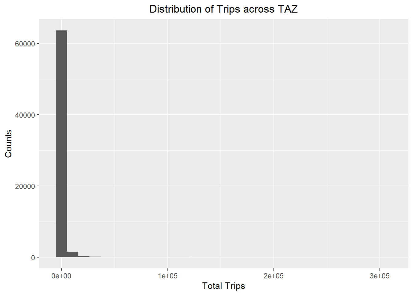
ggplot(data = flow_data2,
       aes(x = TOTAL_TRIPS)) +
  geom_histogram() +
  labs(title = "Distribution of Trips across TAZ",
       x = "Total Trips",
       y = "Counts") +
  theme(plot.title = element_text(hjust = 0.5))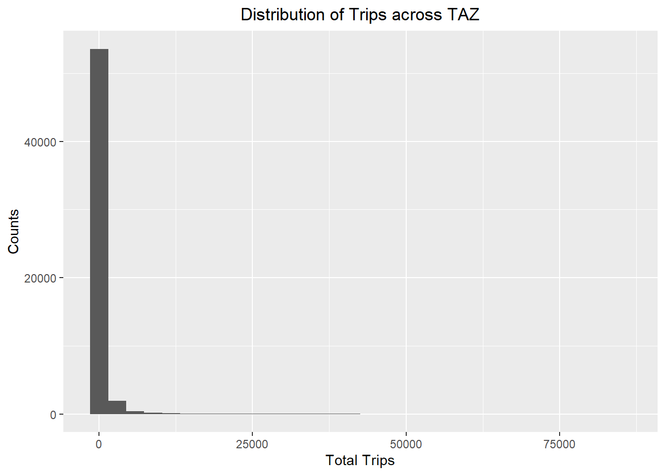
ggplot(data = flow_data3,
       aes(x = TOTAL_TRIPS)) +
  geom_histogram() +
  labs(title = "Distribution of Trips across TAZ",
       x = "Total Trips",
       y = "Counts") +
  theme(plot.title = element_text(hjust = 0.5))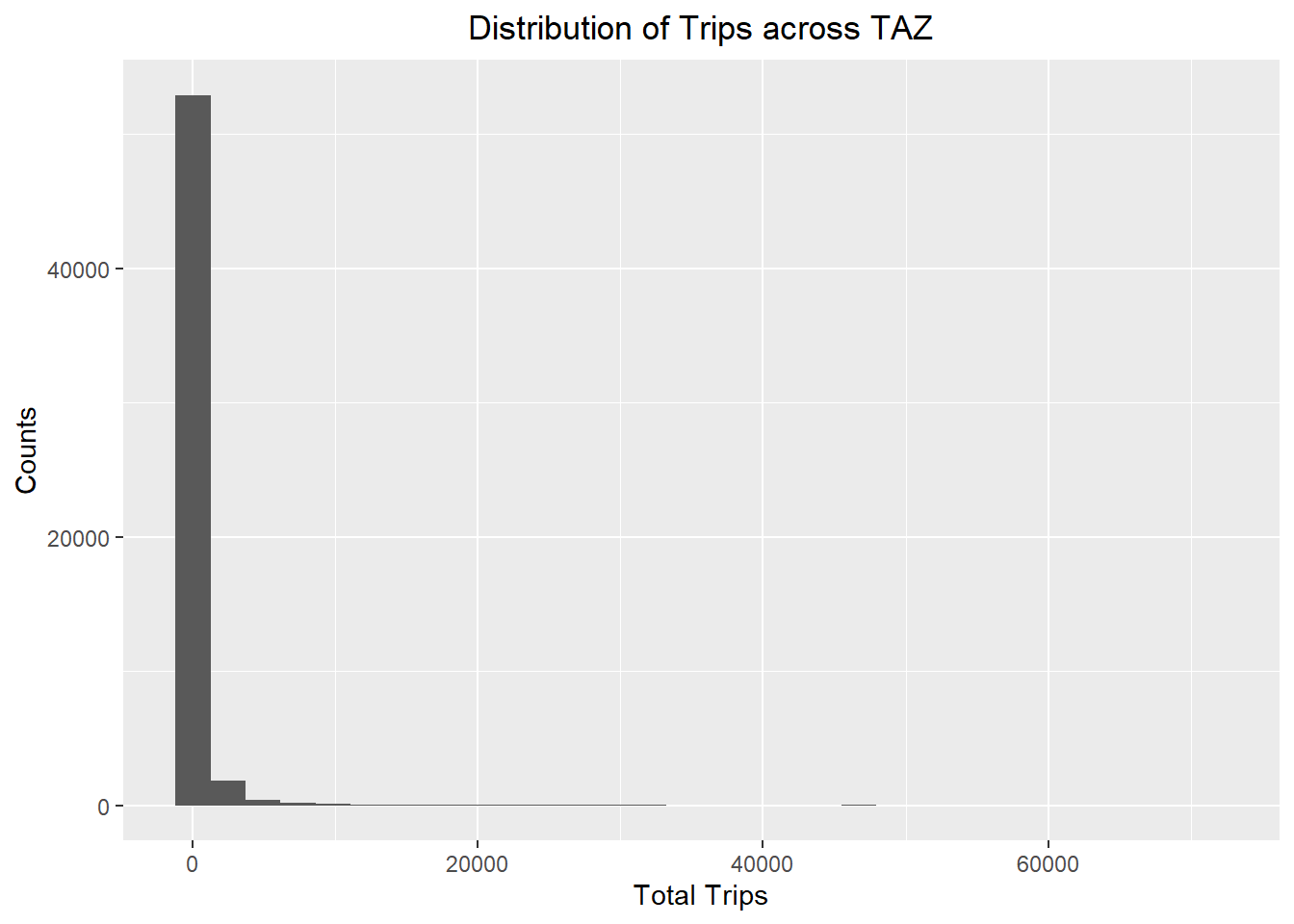
ggplot(data = flow_data4,
       aes(x = TOTAL_TRIPS)) +
  geom_histogram() +
  labs(title = "Distribution of Trips across TAZ",
       x = "Total Trips",
       y = "Counts") +
  theme(plot.title = element_text(hjust = 0.5))
ggplot(data = flow_data5,
       aes(x = TOTAL_TRIPS)) +
  geom_histogram() +
  labs(title = "Distribution of Trips across TAZ",
       x = "Total Trips",
       y = "Counts") +
  theme(plot.title = element_text(hjust = 0.5))
ggplot(data = flow_data6,
       aes(x = TOTAL_TRIPS)) +
  geom_histogram() +
  labs(title = "Distribution of Trips across TAZ",
       x = "Total Trips",
       y = "Counts") +
  theme(plot.title = element_text(hjust = 0.5))
ggplot(data = flow_data7,
       aes(x = TOTAL_TRIPS)) +
  geom_histogram() +
  labs(title = "Distribution of Trips across TAZ",
       x = "Total Trips",
       y = "Counts") +
  theme(plot.title = element_text(hjust = 0.5))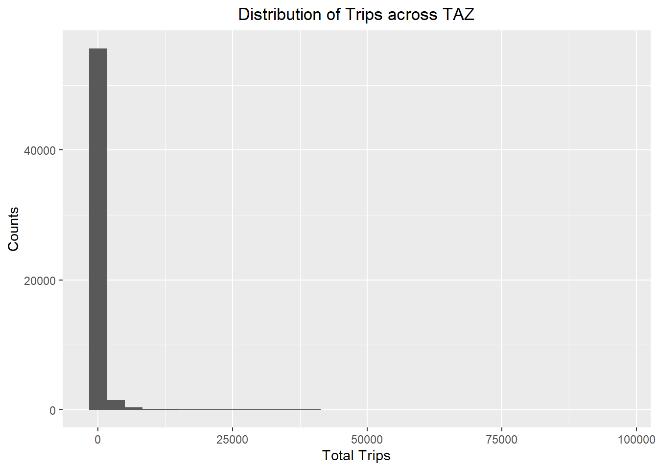
ggplot(data = flow_data8,
       aes(x = TOTAL_TRIPS)) +
  geom_histogram() +
  labs(title = "Distribution of Trips across TAZ",
       x = "Total Trips",
       y = "Counts") +
  theme(plot.title = element_text(hjust = 0.5))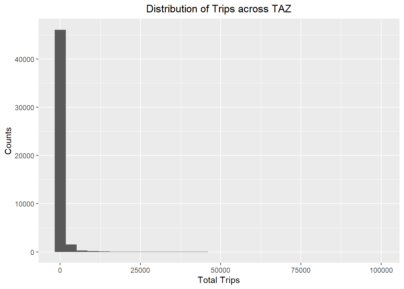
All the distributions are left-skewed and do not resemble a normal distribution.
Visualising with Linear Regression Line
Visualise the relationship between the dependent variable and key independent variable i.e. dist of SIM. Setting the method as lm within geom_smooth() fits a linear regression line to the data.
ggplot(data = flow_data,
       aes(x = dist,
           y = TOTAL_TRIPS)) +
  geom_point() +
  geom_smooth(method = lm) +
  labs(title = "Relationship between Distance and Total Trips",
       x = "Distance",
       y = "Total Trips") +
  theme(plot.title = element_text(hjust = 0.5))
ggplot(data = flow_data2,
       aes(x = dist,
           y = TOTAL_TRIPS)) +
  geom_point() +
  geom_smooth(method = lm) +
  labs(title = "Relationship between Distance and Total Trips",
       x = "Distance",
       y = "Total Trips") +
  theme(plot.title = element_text(hjust = 0.5))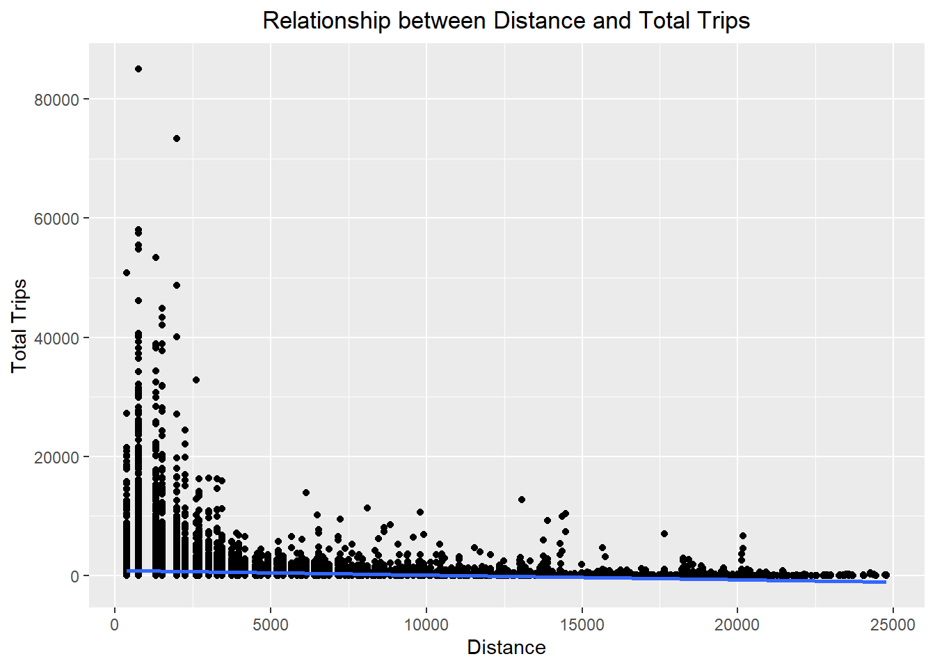
ggplot(data = flow_data3,
       aes(x = dist,
           y = TOTAL_TRIPS)) +
  geom_point() +
  geom_smooth(method = lm) +
  labs(title = "Relationship between Distance and Total Trips",
       x = "Distance",
       y = "Total Trips") +
  theme(plot.title = element_text(hjust = 0.5))
ggplot(data = flow_data4,
       aes(x = dist,
           y = TOTAL_TRIPS)) +
  geom_point() +
  geom_smooth(method = lm) +
  labs(title = "Relationship between Distance and Total Trips",
       x = "Distance",
       y = "Total Trips") +
  theme(plot.title = element_text(hjust = 0.5))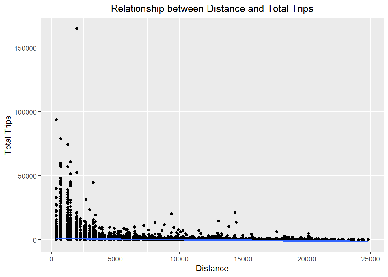
ggplot(data = flow_data5,
       aes(x = dist,
           y = TOTAL_TRIPS)) +
  geom_point() +
  geom_smooth(method = lm) +
  labs(title = "Relationship between Distance and Total Trips",
       x = "Distance",
       y = "Total Trips") +
  theme(plot.title = element_text(hjust = 0.5))
ggplot(data = flow_data6,
       aes(x = dist,
           y = TOTAL_TRIPS)) +
  geom_point() +
  geom_smooth(method = lm) +
  labs(title = "Relationship between Distance and Total Trips",
       x = "Distance",
       y = "Total Trips") +
  theme(plot.title = element_text(hjust = 0.5))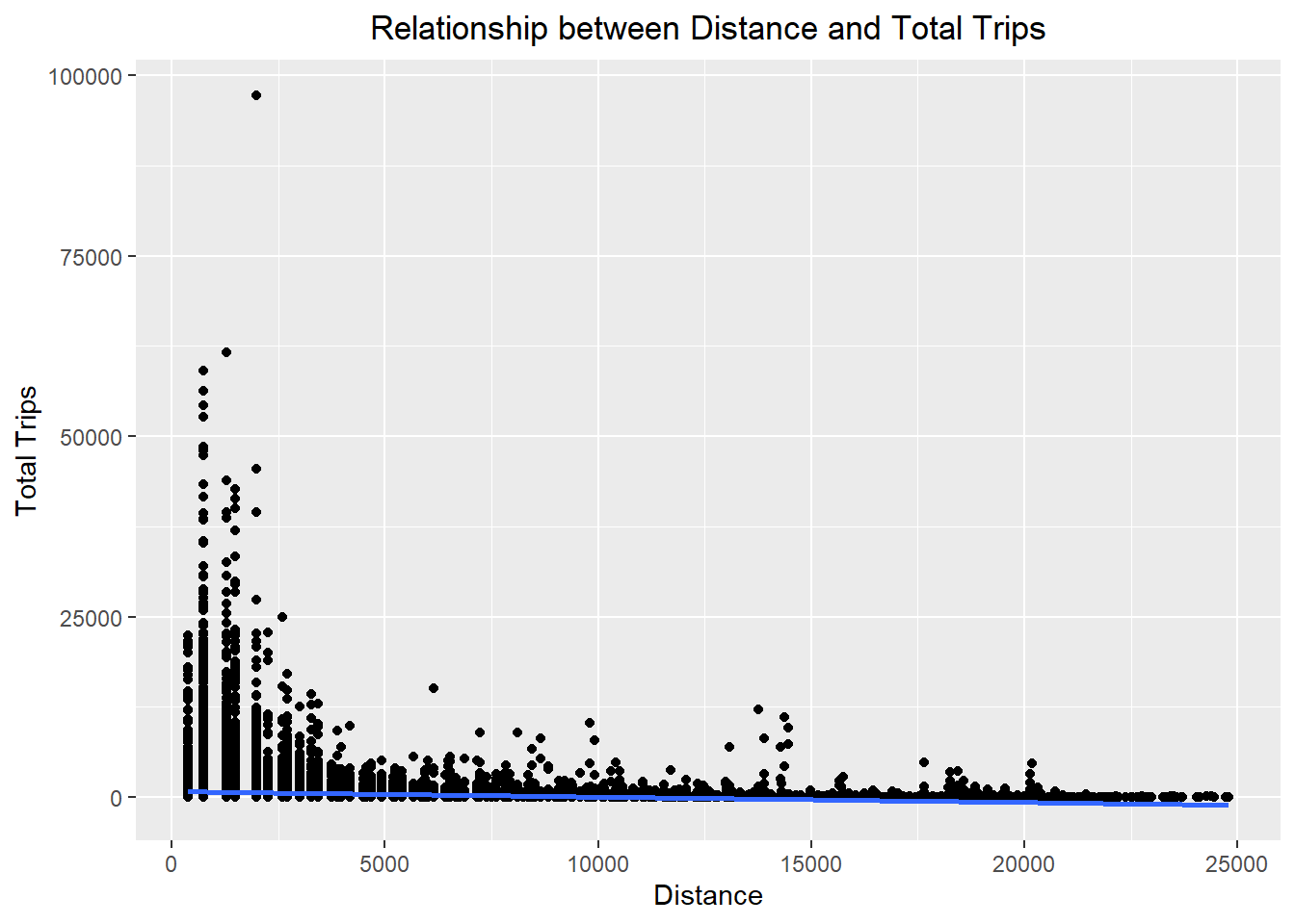
ggplot(data = flow_data7,
       aes(x = dist,
           y = TOTAL_TRIPS)) +
  geom_point() +
  geom_smooth(method = lm) +
  labs(title = "Relationship between Distance and Total Trips",
       x = "Distance",
       y = "Total Trips") +
  theme(plot.title = element_text(hjust = 0.5))
ggplot(data = flow_data8,
       aes(x = dist,
           y = TOTAL_TRIPS)) +
  geom_point() +
  geom_smooth(method = lm) +
  labs(title = "Relationship between Distance and Total Trips",
       x = "Distance",
       y = "Total Trips") +
  theme(plot.title = element_text(hjust = 0.5))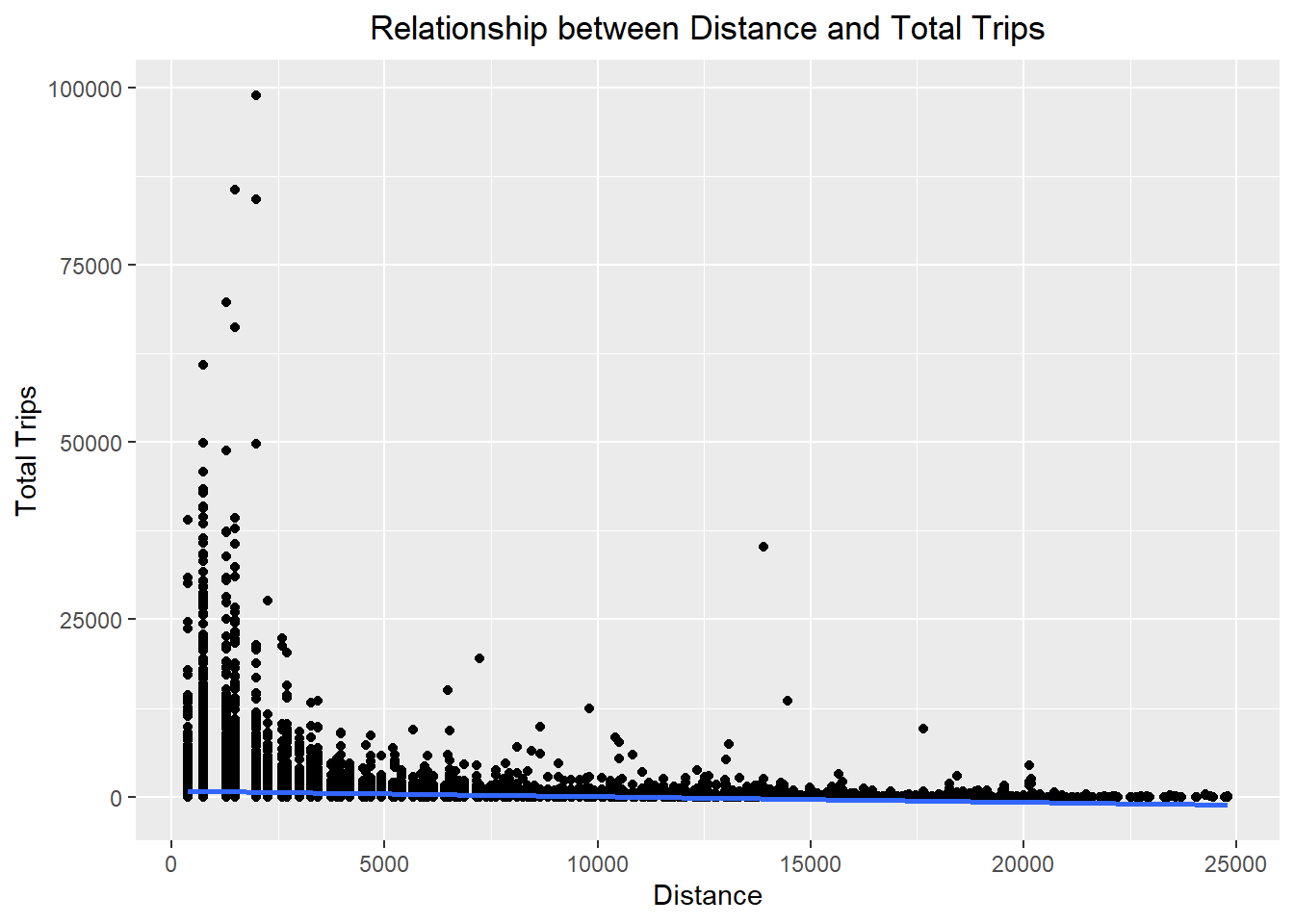
Visualising Scatterplot after Log Transformation
ggplot(data = flow_data,
       aes(x = log(dist),
           y = log(TOTAL_TRIPS))) +
  geom_point() +
  geom_smooth(method = lm) +
  labs(title = "Relationship between Log Distance and Log Total Trips",
       x = "Log Distance",
       y = "Log Total Trips") +
  theme(plot.title = element_text(hjust = 0.5))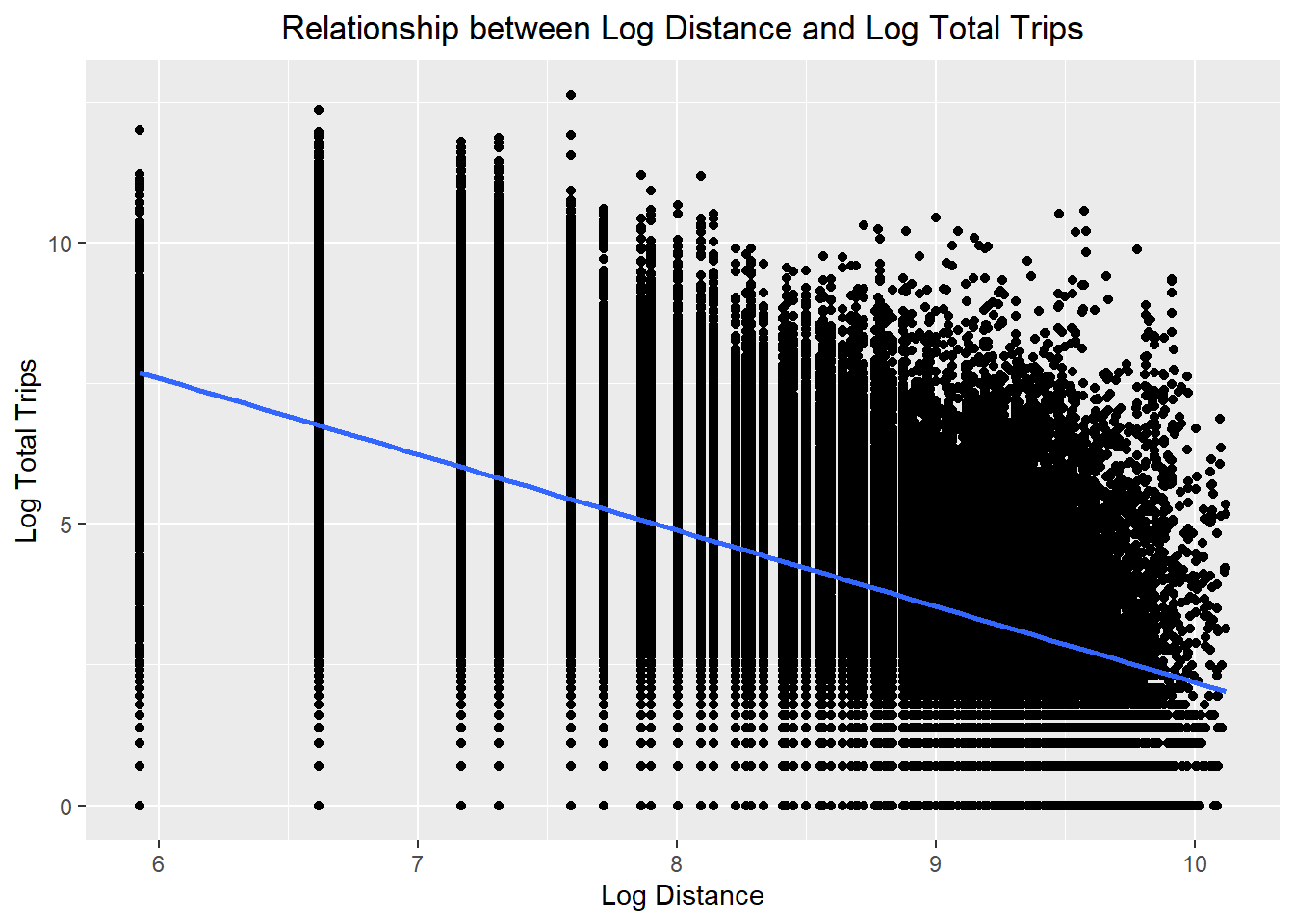
ggplot(data = flow_data2,
       aes(x = log(dist),
           y = log(TOTAL_TRIPS))) +
  geom_point() +
  geom_smooth(method = lm) +
  labs(title = "Relationship between Log Distance and Log Total Trips",
       x = "Log Distance",
       y = "Log Total Trips") +
  theme(plot.title = element_text(hjust = 0.5))
ggplot(data = flow_data3,
       aes(x = log(dist),
           y = log(TOTAL_TRIPS))) +
  geom_point() +
  geom_smooth(method = lm) +
  labs(title = "Relationship between Log Distance and Log Total Trips",
       x = "Log Distance",
       y = "Log Total Trips") +
  theme(plot.title = element_text(hjust = 0.5))
ggplot(data = flow_data4,
       aes(x = log(dist),
           y = log(TOTAL_TRIPS))) +
  geom_point() +
  geom_smooth(method = lm) +
  labs(title = "Relationship between Log Distance and Log Total Trips",
       x = "Log Distance",
       y = "Log Total Trips") +
  theme(plot.title = element_text(hjust = 0.5))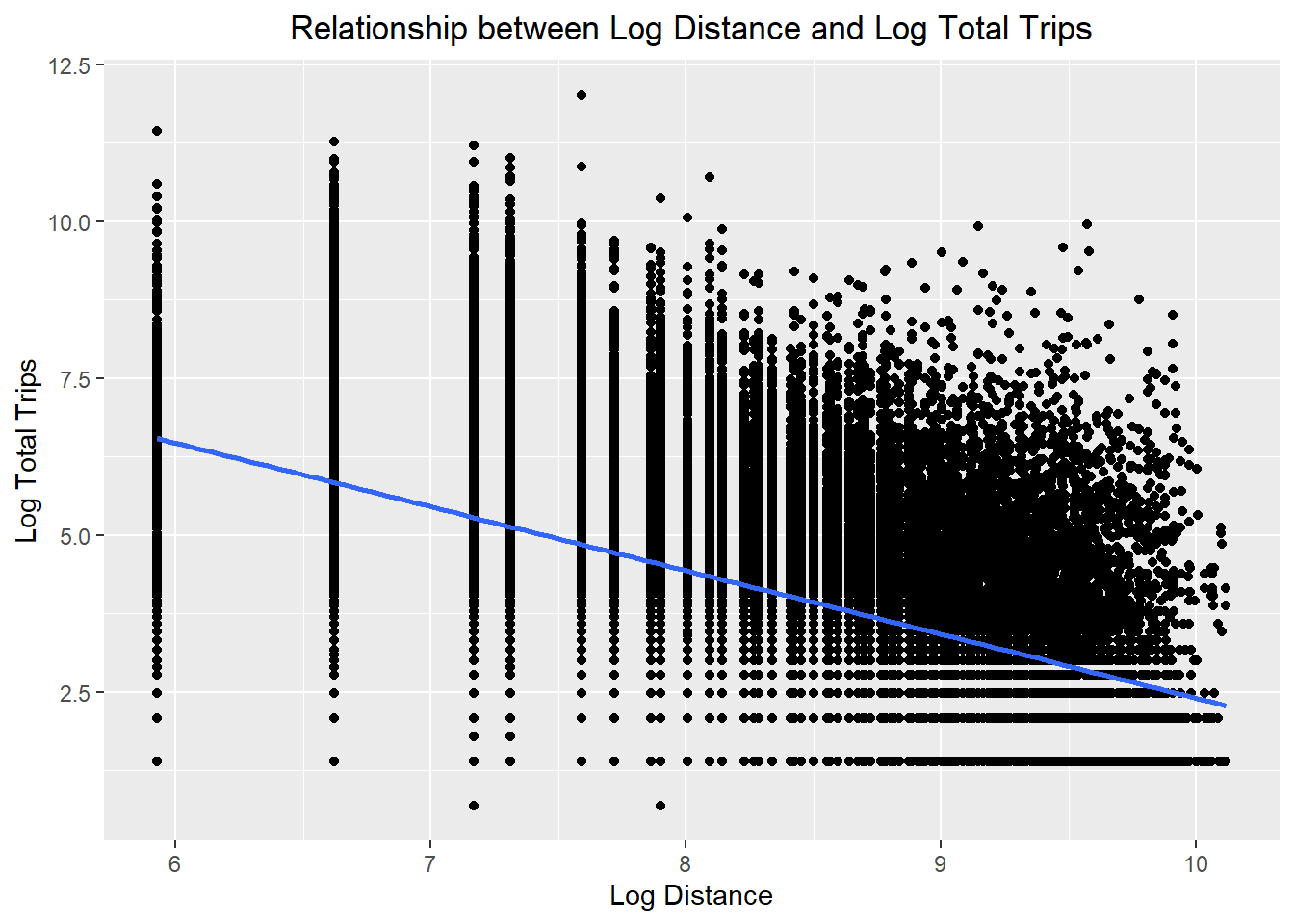
ggplot(data = flow_data5,
       aes(x = log(dist),
           y = log(TOTAL_TRIPS))) +
  geom_point() +
  geom_smooth(method = lm) +
  labs(title = "Relationship between Log Distance and Log Total Trips",
       x = "Log Distance",
       y = "Log Total Trips") +
  theme(plot.title = element_text(hjust = 0.5))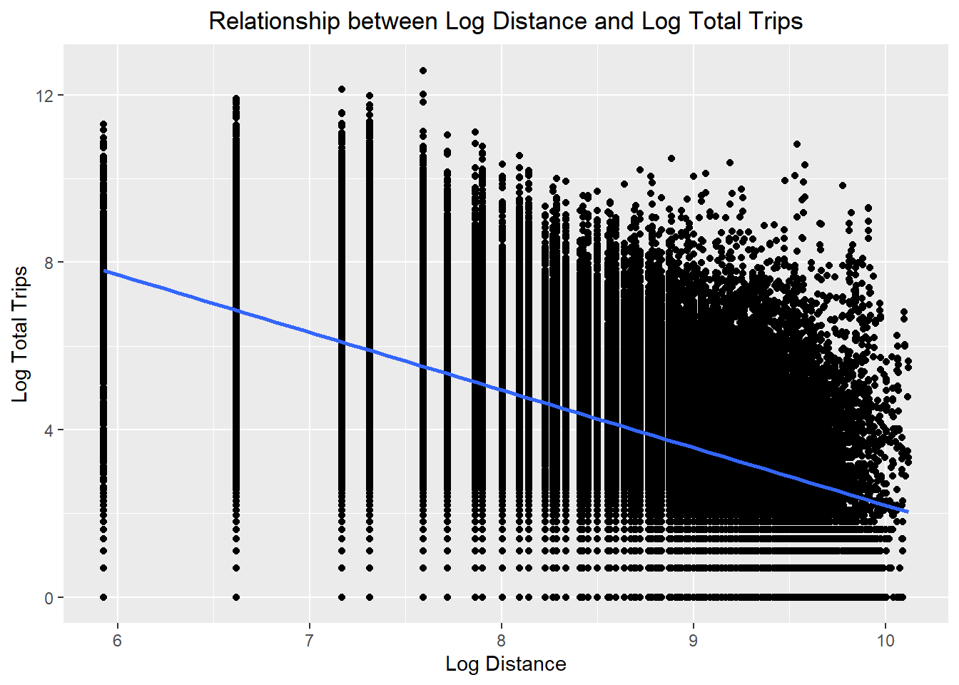
ggplot(data = flow_data6,
       aes(x = log(dist),
           y = log(TOTAL_TRIPS))) +
  geom_point() +
  geom_smooth(method = lm) +
  labs(title = "Relationship between Log Distance and Log Total Trips",
       x = "Log Distance",
       y = "Log Total Trips") +
  theme(plot.title = element_text(hjust = 0.5))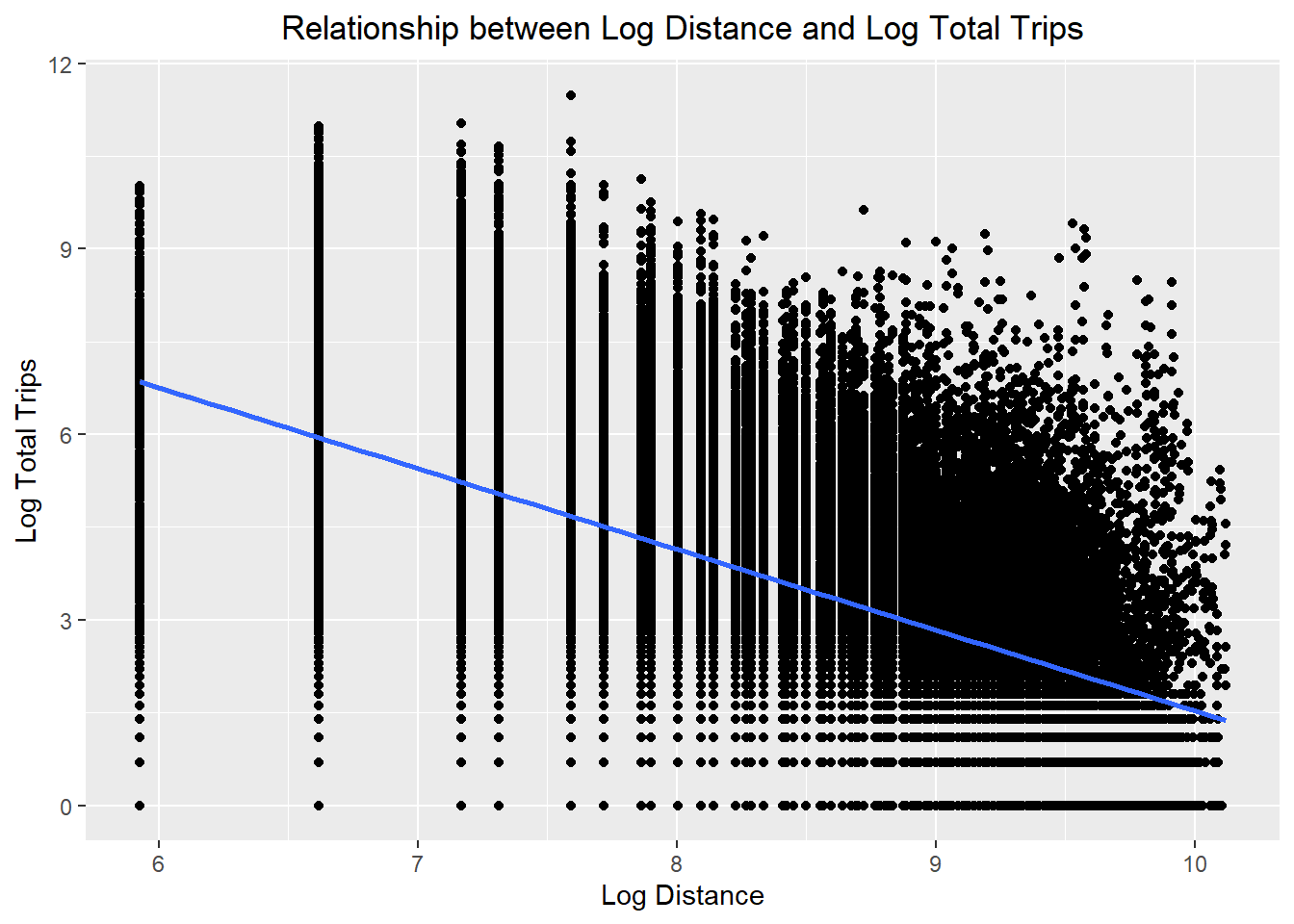
ggplot(data = flow_data7,
       aes(x = log(dist),
           y = log(TOTAL_TRIPS))) +
  geom_point() +
  geom_smooth(method = lm) +
  labs(title = "Relationship between Log Distance and Log Total Trips",
       x = "Log Distance",
       y = "Log Total Trips") +
  theme(plot.title = element_text(hjust = 0.5))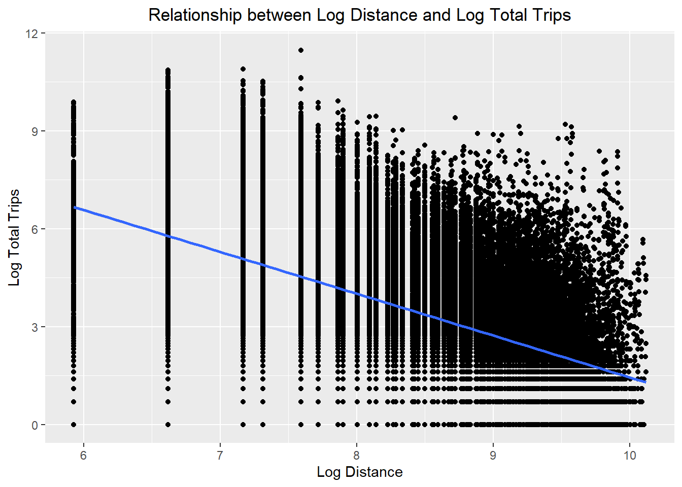
ggplot(data = flow_data8,
       aes(x = log(dist),
           y = log(TOTAL_TRIPS))) +
  geom_point() +
  geom_smooth(method = lm) +
  labs(title = "Relationship between Log Distance and Log Total Trips",
       x = "Log Distance",
       y = "Log Total Trips") +
  theme(plot.title = element_text(hjust = 0.5))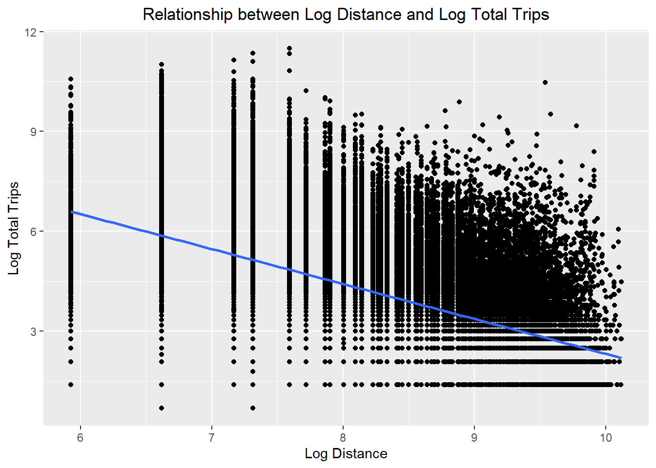
- The relationships are still non-linear but they are less skewed than before
Poisson Regression
Now we need to transform the zero values so that log transformation can be done correctly for the explanatory variables according to Poisson Regression.
Changing zero values
flow_data <- flow_data %>%
  mutate_at(vars(ends_with("_count")), ~ ifelse(. == 0, 0.99, .))

flow_data2<- flow_data2 %>%
  mutate_at(vars(ends_with("_count")), ~ ifelse(. == 0, 0.99, .))

flow_data3 <- flow_data3 %>%
  mutate_at(vars(ends_with("_count")), ~ ifelse(. == 0, 0.99, .))

flow_data4 <- flow_data4 %>%
  mutate_at(vars(ends_with("_count")), ~ ifelse(. == 0, 0.99, .))

flow_data5 <- flow_data5 %>%
  mutate_at(vars(ends_with("_count")), ~ ifelse(. == 0, 0.99, .))

flow_data6 <- flow_data6 %>%
  mutate_at(vars(ends_with("_count")), ~ ifelse(. == 0, 0.99, .))

flow_data7 <- flow_data7 %>%
  mutate_at(vars(ends_with("_count")), ~ ifelse(. == 0, 0.99, .))

flow_data8 <- flow_data8 %>%
  mutate_at(vars(ends_with("_count")), ~ ifelse(. == 0, 0.99, .))
References
Jacek Chmielewski and Jan Kempa, 2020. Hexagonal Zones in Transport Demand Models, International Congress on Engineering – Engineering for Evolution. Volume 2020.